Graph Neural Networks Demystified: From Theory to PyTorch Geometric

Introduction

In our previous posts, we built a Knowledge Graph with Neo4j and analyzed it using Graph Algorithms like PageRank. These methods are powerful, but they are often limited to “shallow” learning.

Enter Graph Neural Networks (GNNs).

GNNs are a class of deep learning models designed to perform inference on data described by graphs. They have revolutionized fields like drug discovery, recommender systems, and traffic prediction.

Why not just use a standard Neural Network?

Standard NNs (like CNNs or RNNs) expect data in a fixed structure (grid or sequence). Graphs are non-Euclidean—they have no fixed order and varying neighbors. GNNs are designed to handle this irregularity.

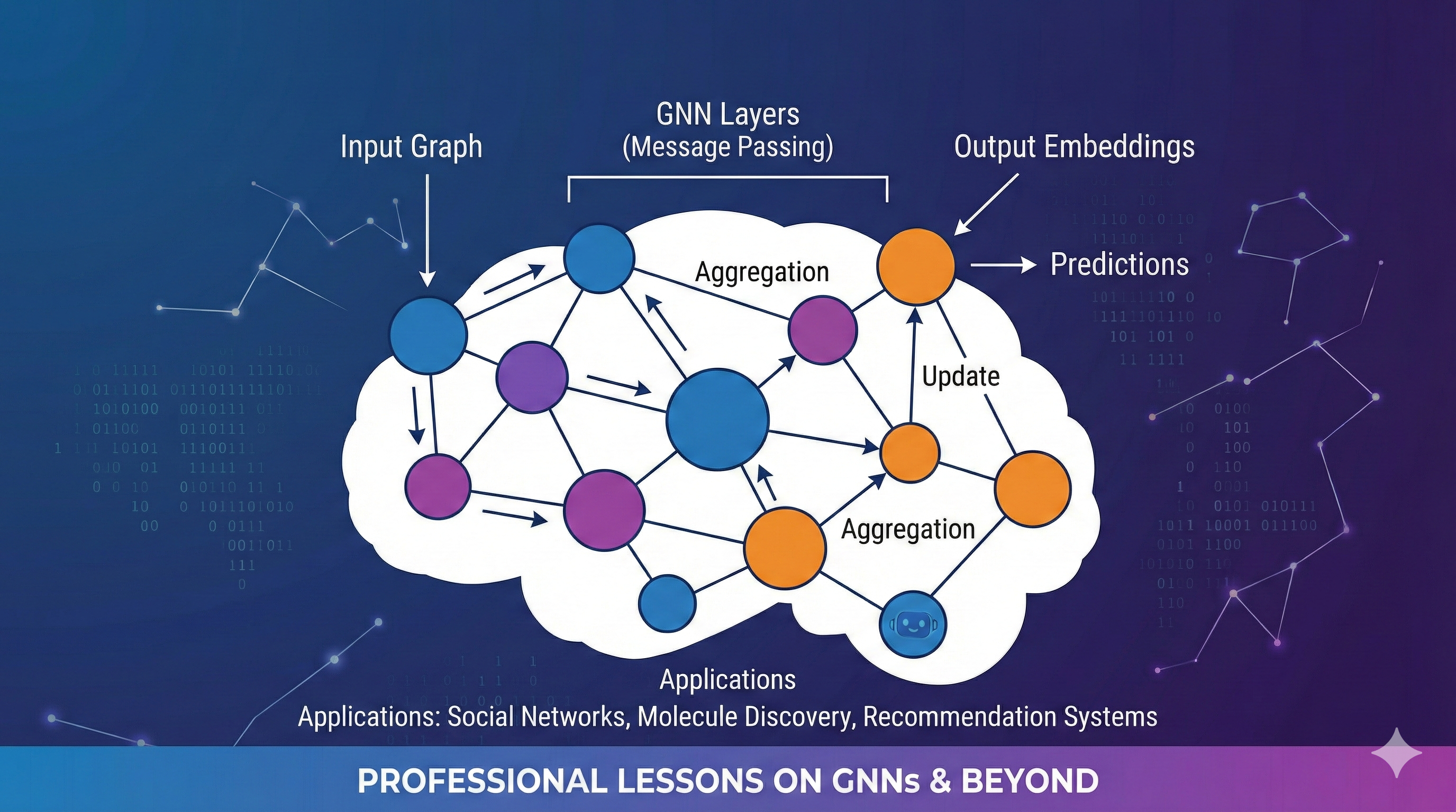
The Core Concept: Message Passing

The magic of GNNs lies in the Message Passing Framework.

For every node in the graph, we:

1. Gather information (messages) from its neighbors.
2. Aggregate these messages (e.g., sum, mean, max).
3. Update the node’s own representation (embedding) based on the aggregated message and its previous state.

Mathematically, for a node $v$, its hidden state $h_v^{(k)}$ at layer $k$ is updated as:

\[h_v^{(k)} = \sigma \left( W^{(k)} \cdot \text{AGG} \left( \{ h_u^{(k-1)} : u \in \mathcal{N}(v) \} \right) \right)\]

Where:

• $\mathcal{N}(v)$ is the set of neighbors of $v$.
• $\text{AGG}$ is a differentiable, permutation-invariant function (like sum or mean).
• $W^{(k)}$ is a learnable weight matrix.
• $\sigma$ is a non-linear activation function (like ReLU).

Visualizing Message Passing

graph TD
    subgraph Layer k-1
    A((A)) --> B((B))
    C((C)) --> B
    D((D)) --> B
    end
    
    subgraph Layer k
    B_new((B'))
    end
    
    B -.->|Message| B_new
    A -.->|Message| B_new
    C -.->|Message| B_new
    D -.->|Message| B_new
    
    style B_new fill:#f9f,stroke:#333,stroke-width:4px

Popular GNN Architectures

1. Graph Convolutional Networks (GCN)

GCNs are the “Hello World” of GNNs. They use a specific aggregation rule that approximates a spectral convolution.

\[h_v^{(k)} = \sigma \left( \sum_{u \in \mathcal{N}(v) \cup \{v\}} \frac{1}{\sqrt{\text{deg}(v)\text{deg}(u)}} W^{(k)} h_u^{(k-1)} \right)\]

2. GraphSAGE (Graph Sample and Aggregate)

GraphSAGE is designed for inductive learning (handling unseen nodes). It learns to aggregate information from a fixed number of sampled neighbors.

3. Graph Attention Networks (GAT)

GAT adds an attention mechanism. Instead of treating all neighbors equally, it learns importance weights $\alpha_{vu}$ for each neighbor.

Hands-On: Node Classification with PyTorch Geometric

Let’s implement a simple GCN using PyTorch Geometric (PyG), the leading library for GNNs.

We’ll use the Cora dataset, a citation network where nodes are papers and edges are citations. The goal is to classify papers into subjects.

Installation

pip install torch torch_geometric

Implementation

import torch
import torch.nn.functional as F
from torch_geometric.nn import GCNConv
from torch_geometric.datasets import Planetoid

# 1. Load the Cora dataset
dataset = Planetoid(root='/tmp/Cora', name='Cora')
data = dataset[0]

print(f'Nodes: {data.num_nodes}')
print(f'Edges: {data.num_edges}')
print(f'Features: {data.num_node_features}')
print(f'Classes: {dataset.num_classes}')

# 2. Define the GCN Model
class GCN(torch.nn.Module):
    def __init__(self):
        super().__init__()
        # Two Graph Convolutional Layers
        self.conv1 = GCNConv(dataset.num_node_features, 16)
        self.conv2 = GCNConv(16, dataset.num_classes)

    def forward(self, data):
        x, edge_index = data.x, data.edge_index

        # Layer 1
        x = self.conv1(x, edge_index)
        x = F.relu(x)
        x = F.dropout(x, training=self.training)

        # Layer 2
        x = self.conv2(x, edge_index)
        
        return F.log_softmax(x, dim=1)

# 3. Train the Model
device = torch.device('cuda' if torch.cuda.is_available() else 'cpu')
model = GCN().to(device)
data = data.to(device)
optimizer = torch.optim.Adam(model.parameters(), lr=0.01, weight_decay=5e-4)

model.train()
for epoch in range(200):
    optimizer.zero_grad()
    out = model(data)
    loss = F.nll_loss(out[data.train_mask], data.y[data.train_mask])
    loss.backward()
    optimizer.step()

# 4. Evaluate
model.eval()
pred = model(data).argmax(dim=1)
correct = (pred[data.test_mask] == data.y[data.test_mask]).sum()
acc = int(correct) / int(data.test_mask.sum())
print(f'Accuracy: {acc:.4f}')

Conclusion

We’ve just scratched the surface of Graph Neural Networks. By leveraging the structure of data, GNNs unlock performance that traditional models can’t match on relational datasets.

Next Steps

Try applying this GCN model to our African Tech Ecosystem graph! You could predict the “Category” of a startup based on its investors and connections.

References

1. PyTorch Geometric Documentation
2. A Gentle Introduction to Graph Neural Networks (Distill)
3. Semi-Supervised Classification with Graph Convolutional Networks (Kipf & Welling)

---

Related Posts:

• Graph Algorithms in Neo4j
• Building a Knowledge Graph with Neo4j and Python

---

Learning from connections. 🧠