Momentum and Adaptive Learning Rates: Accelerating Deep Learning Optimization

Introduction

While vanilla gradient descent laid the foundation for modern machine learning, training deep neural networks requires more sophisticated optimization techniques. In this comprehensive guide, we’ll explore momentum-based methods and adaptive learning rate algorithms that have become the backbone of deep learning optimization.

Key Insight

The journey from SGD to Adam represents one of the most impactful advances in deep learning, reducing training time from weeks to hours for many architectures.

The Problem with Vanilla Gradient Descent

Standard gradient descent suffers from several critical limitations:

1. Slow convergence in ravines (regions where the surface curves more steeply in one dimension)
2. Oscillation around local minima
3. Uniform learning rates across all parameters
4. Sensitivity to learning rate selection

Let’s visualize the optimization landscape:

graph TD
    A[Start: Random Initialization] --> B{Gradient Descent Type}
    B -->|Vanilla GD| C[Slow, Oscillating Path]
    B -->|Momentum| D[Faster, Smoother Path]
    B -->|Adam| E[Adaptive, Optimal Path]
    
    C --> F[Local Minimum]
    D --> F
    E --> F
    
    style C fill:#ff6b6b
    style D fill:#ffd93d
    style E fill:#6bcf7f

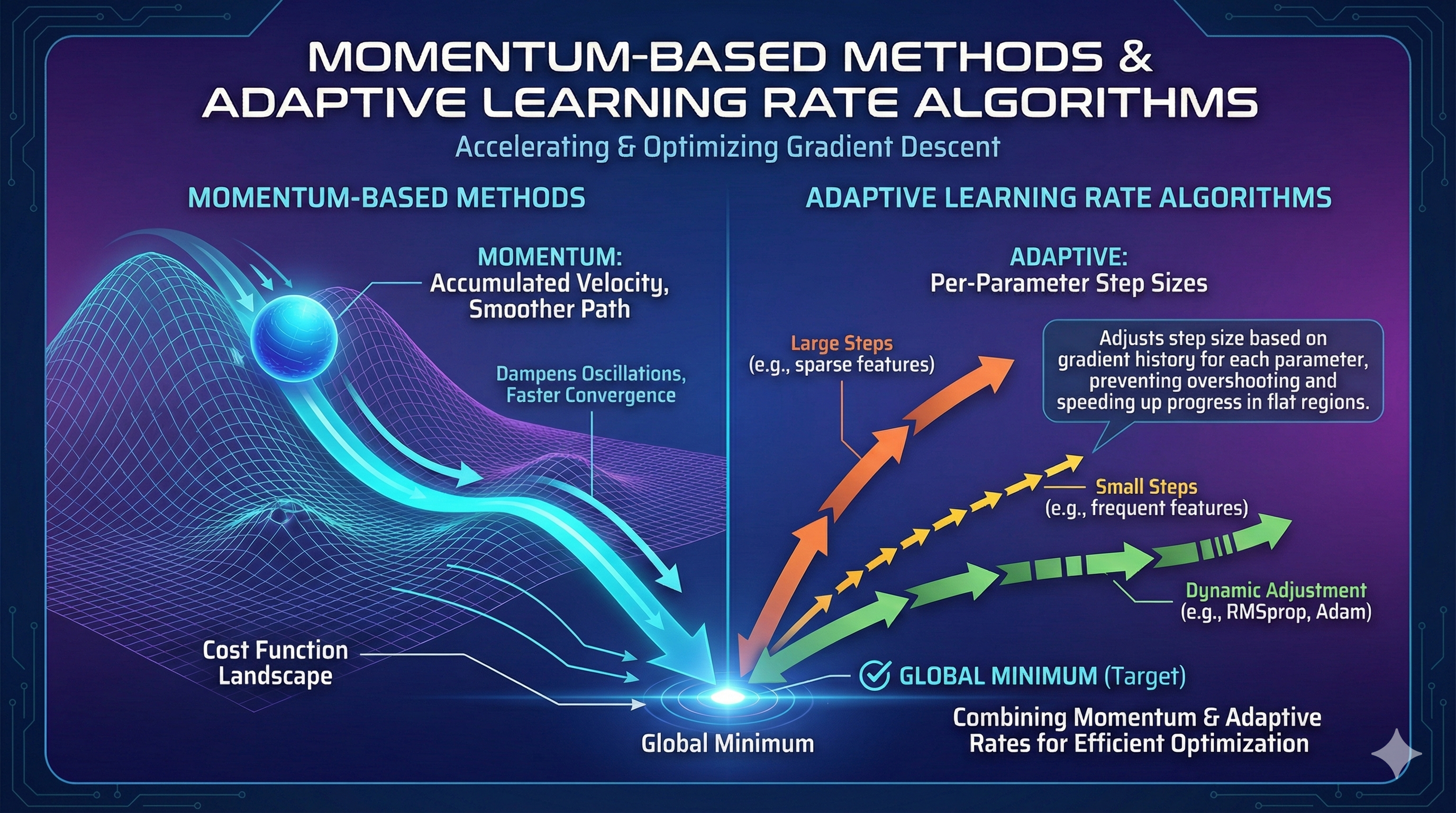
Momentum: Physics-Inspired Optimization

The Core Concept

Momentum borrows from physics: imagine a ball rolling down a hill. It accumulates velocity as it descends, allowing it to:

• Accelerate through flat regions
• Dampen oscillations in steep ravines
• Escape shallow local minima

Mathematical Formulation

The momentum update rule introduces a velocity term $v$:

\[\begin{aligned} v_t &= \beta v_{t-1} + \nabla J(\theta_{t-1}) \\ \theta_t &= \theta_{t-1} - \alpha v_t \end{aligned}\]

Where:

• $v_t$ is the velocity at time $t$
• $\beta$ is the momentum coefficient (typically 0.9)
• $\alpha$ is the learning rate
• $\nabla J(\theta)$ is the gradient

Nesterov Accelerated Gradient (NAG)

Nesterov momentum improves upon standard momentum by looking ahead:

\[\begin{aligned} v_t &= \beta v_{t-1} + \nabla J(\theta_{t-1} - \beta v_{t-1}) \\ \theta_t &= \theta_{t-1} - \alpha v_t \end{aligned}\]

This “look-ahead” gradient provides better convergence properties.

Python Implementation

import numpy as np
from typing import Tuple, List

class MomentumOptimizer:
    """
    Gradient descent with momentum optimization.
    
    Attributes:
        learning_rate: Step size for parameter updates
        momentum: Momentum coefficient (beta)
        velocity: Accumulated gradient history
    """
    
    def __init__(self, learning_rate: float = 0.01, momentum: float = 0.9):
        self.learning_rate = learning_rate
        self.momentum = momentum
        self.velocity = None
    
    def update(self, params: np.ndarray, gradients: np.ndarray) -> np.ndarray:
        """
        Update parameters using momentum.
        
        Args:
            params: Current parameter values
            gradients: Computed gradients
            
        Returns:
            Updated parameters
        """
        # Initialize velocity on first call
        if self.velocity is None:
            self.velocity = np.zeros_like(params)
        
        # Update velocity: v = beta * v + grad
        self.velocity = self.momentum * self.velocity + gradients
        
        # Update parameters: theta = theta - lr * v
        params = params - self.learning_rate * self.velocity
        
        return params


class NesterovOptimizer:
    """Nesterov Accelerated Gradient optimizer."""
    
    def __init__(self, learning_rate: float = 0.01, momentum: float = 0.9):
        self.learning_rate = learning_rate
        self.momentum = momentum
        self.velocity = None
    
    def update(self, params: np.ndarray, gradient_fn) -> np.ndarray:
        """
        Update parameters using Nesterov momentum.
        
        Args:
            params: Current parameter values
            gradient_fn: Function that computes gradients at given params
            
        Returns:
            Updated parameters
        """
        if self.velocity is None:
            self.velocity = np.zeros_like(params)
        
        # Look-ahead step
        params_ahead = params - self.momentum * self.velocity
        
        # Compute gradient at look-ahead position
        gradients = gradient_fn(params_ahead)
        
        # Update velocity and parameters
        self.velocity = self.momentum * self.velocity + gradients
        params = params - self.learning_rate * self.velocity
        
        return params


# Example usage
def rosenbrock_gradient(params):
    """Gradient of the Rosenbrock function."""
    x, y = params
    dx = -400 * x * (y - x**2) - 2 * (1 - x)
    dy = 200 * (y - x**2)
    return np.array([dx, dy])

# Initialize optimizers
momentum_opt = MomentumOptimizer(learning_rate=0.001, momentum=0.9)
nesterov_opt = NesterovOptimizer(learning_rate=0.001, momentum=0.9)

# Starting point
params = np.array([-1.0, 1.0])

# Run optimization
for i in range(100):
    gradients = rosenbrock_gradient(params)
    params = momentum_opt.update(params, gradients)
    
    if i % 20 == 0:
        print(f"Iteration {i}: params = {params}")

Adaptive Learning Rate Methods

The Motivation

Different parameters often require different learning rates:

• Sparse features need larger updates (they update infrequently)
• Dense features need smaller updates (they update constantly)
• Deep layers may need different rates than shallow layers

AdaGrad: Adaptive Gradient Algorithm

AdaGrad adapts the learning rate for each parameter based on historical gradients:

\[\theta_{t,i} = \theta_{t-1,i} - \frac{\alpha}{\sqrt{G_{t,i} + \epsilon}} \cdot g_{t,i}\]

Where $G_{t,i}$ is the sum of squared gradients for parameter $i$ up to time $t$:

\[G_{t,i} = \sum_{\tau=1}^{t} g_{\tau,i}^2\]

Warning: AdaGrad Limitation

The accumulated squared gradients grow monotonically, causing the learning rate to eventually become infinitesimally small. This makes AdaGrad unsuitable for training deep networks.

RMSprop: Root Mean Square Propagation

RMSprop fixes AdaGrad’s diminishing learning rate problem using an exponentially weighted moving average:

\[\begin{aligned} E[g^2]_t &= \beta E[g^2]_{t-1} + (1-\beta) g_t^2 \\ \theta_t &= \theta_{t-1} - \frac{\alpha}{\sqrt{E[g^2]_t + \epsilon}} \cdot g_t \end{aligned}\]

Adam: Adaptive Moment Estimation

Adam combines the best of momentum and RMSprop, maintaining both:

1. First moment (mean) of gradients (like momentum)
2. Second moment (uncentered variance) of gradients (like RMSprop)

The complete Adam update:

\[\begin{aligned} m_t &= \beta_1 m_{t-1} + (1-\beta_1) g_t \\ v_t &= \beta_2 v_{t-1} + (1-\beta_2) g_t^2 \\ \hat{m}_t &= \frac{m_t}{1-\beta_1^t} \\ \hat{v}_t &= \frac{v_t}{1-\beta_2^t} \\ \theta_t &= \theta_{t-1} - \frac{\alpha}{\sqrt{\hat{v}_t} + \epsilon} \cdot \hat{m}_t \end{aligned}\]

Default hyperparameters: $\beta_1 = 0.9$, $\beta_2 = 0.999$, $\epsilon = 10^{-8}$

Complete Implementation

class AdamOptimizer:
    """
    Adam (Adaptive Moment Estimation) optimizer.
    
    Combines momentum and RMSprop for robust optimization.
    """
    
    def __init__(
        self, 
        learning_rate: float = 0.001,
        beta1: float = 0.9,
        beta2: float = 0.999,
        epsilon: float = 1e-8
    ):
        self.learning_rate = learning_rate
        self.beta1 = beta1
        self.beta2 = beta2
        self.epsilon = epsilon
        
        # Initialize moment estimates
        self.m = None  # First moment (mean)
        self.v = None  # Second moment (uncentered variance)
        self.t = 0     # Time step
    
    def update(self, params: np.ndarray, gradients: np.ndarray) -> np.ndarray:
        """
        Update parameters using Adam algorithm.
        
        Args:
            params: Current parameter values
            gradients: Computed gradients
            
        Returns:
            Updated parameters
        """
        # Initialize moments on first call
        if self.m is None:
            self.m = np.zeros_like(params)
            self.v = np.zeros_like(params)
        
        self.t += 1
        
        # Update biased first moment estimate
        self.m = self.beta1 * self.m + (1 - self.beta1) * gradients
        
        # Update biased second raw moment estimate
        self.v = self.beta2 * self.v + (1 - self.beta2) * (gradients ** 2)
        
        # Compute bias-corrected first moment estimate
        m_hat = self.m / (1 - self.beta1 ** self.t)
        
        # Compute bias-corrected second raw moment estimate
        v_hat = self.v / (1 - self.beta2 ** self.t)
        
        # Update parameters
        params = params - self.learning_rate * m_hat / (np.sqrt(v_hat) + self.epsilon)
        
        return params


class RMSpropOptimizer:
    """RMSprop optimizer with exponentially decaying average of squared gradients."""
    
    def __init__(
        self,
        learning_rate: float = 0.001,
        decay_rate: float = 0.9,
        epsilon: float = 1e-8
    ):
        self.learning_rate = learning_rate
        self.decay_rate = decay_rate
        self.epsilon = epsilon
        self.cache = None
    
    def update(self, params: np.ndarray, gradients: np.ndarray) -> np.ndarray:
        """Update parameters using RMSprop."""
        if self.cache is None:
            self.cache = np.zeros_like(params)
        
        # Accumulate squared gradients
        self.cache = self.decay_rate * self.cache + (1 - self.decay_rate) * (gradients ** 2)
        
        # Update parameters
        params = params - self.learning_rate * gradients / (np.sqrt(self.cache) + self.epsilon)
        
        return params

Comparative Analysis

Convergence Speed Comparison

graph LR
    A[Optimization Algorithms] --> B[SGD]
    A --> C[Momentum]
    A --> D[RMSprop]
    A --> E[Adam]
    
    B --> F[Baseline Speed]
    C --> G[2-3x Faster]
    D --> H[3-5x Faster]
    E --> I[5-10x Faster]
    
    style B fill:#ff6b6b
    style C fill:#ffd93d
    style D fill:#95e1d3
    style E fill:#6bcf7f

When to Use Each Optimizer

Optimizer	Best For	Pros	Cons
SGD	Convex problems, simple models	Simple, well-understood	Slow, requires tuning
Momentum	Deep networks, ravines	Faster than SGD, smooth	Still needs LR tuning
RMSprop	RNNs, non-stationary problems	Adaptive LR	Can be unstable
Adam	Most deep learning tasks	Fast, robust, minimal tuning	Can overfit, memory intensive

Tip: Optimizer Selection

Start with Adam for rapid prototyping. If you have time for hyperparameter tuning, SGD with momentum often achieves better final performance on vision tasks.

Advanced Techniques

Learning Rate Scheduling

Even with adaptive optimizers, learning rate schedules improve performance:

class CosineAnnealingScheduler:
    """Cosine annealing learning rate schedule."""
    
    def __init__(self, initial_lr: float, T_max: int, eta_min: float = 0):
        self.initial_lr = initial_lr
        self.T_max = T_max
        self.eta_min = eta_min
    
    def get_lr(self, epoch: int) -> float:
        """Get learning rate for current epoch."""
        return self.eta_min + (self.initial_lr - self.eta_min) * \
               (1 + np.cos(np.pi * epoch / self.T_max)) / 2


class StepDecayScheduler:
    """Step decay learning rate schedule."""
    
    def __init__(self, initial_lr: float, drop_rate: float = 0.5, epochs_drop: int = 10):
        self.initial_lr = initial_lr
        self.drop_rate = drop_rate
        self.epochs_drop = epochs_drop
    
    def get_lr(self, epoch: int) -> float:
        """Get learning rate for current epoch."""
        return self.initial_lr * (self.drop_rate ** (epoch // self.epochs_drop))

Gradient Clipping

Prevent exploding gradients in RNNs and transformers:

def clip_gradients(gradients: np.ndarray, max_norm: float = 5.0) -> np.ndarray:
    """
    Clip gradients by global norm.
    
    Args:
        gradients: Gradient array
        max_norm: Maximum allowed norm
        
    Returns:
        Clipped gradients
    """
    total_norm = np.linalg.norm(gradients)
    
    if total_norm > max_norm:
        gradients = gradients * (max_norm / total_norm)
    
    return gradients

Practical Training Loop

Here’s a complete training loop incorporating these concepts:

def train_model(
    model,
    X_train: np.ndarray,
    y_train: np.ndarray,
    epochs: int = 100,
    batch_size: int = 32,
    optimizer_type: str = 'adam'
):
    """
    Complete training loop with modern optimization.
    
    Args:
        model: Neural network model
        X_train: Training features
        y_train: Training labels
        epochs: Number of training epochs
        batch_size: Mini-batch size
        optimizer_type: 'sgd', 'momentum', 'rmsprop', or 'adam'
    """
    # Initialize optimizer
    optimizers = {
        'sgd': lambda: MomentumOptimizer(learning_rate=0.01, momentum=0.0),
        'momentum': lambda: MomentumOptimizer(learning_rate=0.01, momentum=0.9),
        'rmsprop': lambda: RMSpropOptimizer(learning_rate=0.001),
        'adam': lambda: AdamOptimizer(learning_rate=0.001)
    }
    optimizer = optimizers[optimizer_type]()
    
    # Learning rate scheduler
    scheduler = CosineAnnealingScheduler(initial_lr=0.001, T_max=epochs)
    
    n_samples = X_train.shape[0]
    history = {'loss': [], 'lr': []}
    
    for epoch in range(epochs):
        # Update learning rate
        current_lr = scheduler.get_lr(epoch)
        optimizer.learning_rate = current_lr
        
        # Shuffle data
        indices = np.random.permutation(n_samples)
        X_shuffled = X_train[indices]
        y_shuffled = y_train[indices]
        
        epoch_loss = 0
        n_batches = n_samples // batch_size
        
        for batch in range(n_batches):
            # Get mini-batch
            start_idx = batch * batch_size
            end_idx = start_idx + batch_size
            X_batch = X_shuffled[start_idx:end_idx]
            y_batch = y_shuffled[start_idx:end_idx]
            
            # Forward pass
            predictions = model.forward(X_batch)
            loss = model.compute_loss(predictions, y_batch)
            
            # Backward pass
            gradients = model.backward(X_batch, y_batch)
            
            # Gradient clipping
            gradients = clip_gradients(gradients, max_norm=5.0)
            
            # Update parameters
            model.params = optimizer.update(model.params, gradients)
            
            epoch_loss += loss
        
        # Log progress
        avg_loss = epoch_loss / n_batches
        history['loss'].append(avg_loss)
        history['lr'].append(current_lr)
        
        if epoch % 10 == 0:
            print(f"Epoch {epoch}/{epochs} - Loss: {avg_loss:.4f} - LR: {current_lr:.6f}")
    
    return history

Conclusion

The evolution from vanilla gradient descent to adaptive optimizers represents a crucial advancement in deep learning:

1. Momentum accelerates convergence and dampens oscillations
2. Adaptive learning rates handle sparse features and varying parameter scales
3. Adam combines both approaches for robust, fast optimization

Key Takeaways

• Use Adam as your default optimizer for most tasks
• Consider SGD + Momentum for final fine-tuning on vision models
• Always use learning rate scheduling for best results
• Apply gradient clipping when training RNNs or transformers

Next Steps

In our next post, we’ll explore second-order optimization methods like L-BFGS and natural gradient descent, and when they outperform first-order methods.

References

1. Kingma & Ba (2014). “Adam: A Method for Stochastic Optimization”
2. Sutskever et al. (2013). “On the importance of initialization and momentum in deep learning”
3. Tieleman & Hinton (2012). “RMSprop: Divide the gradient by a running average”
4. Ruder (2016). “An overview of gradient descent optimization algorithms”

---

Related Posts:

• Introduction to Gradient Descent
• Second-Order Optimization Methods