Second-Order Optimization Methods: Beyond Gradient Descent

Introduction

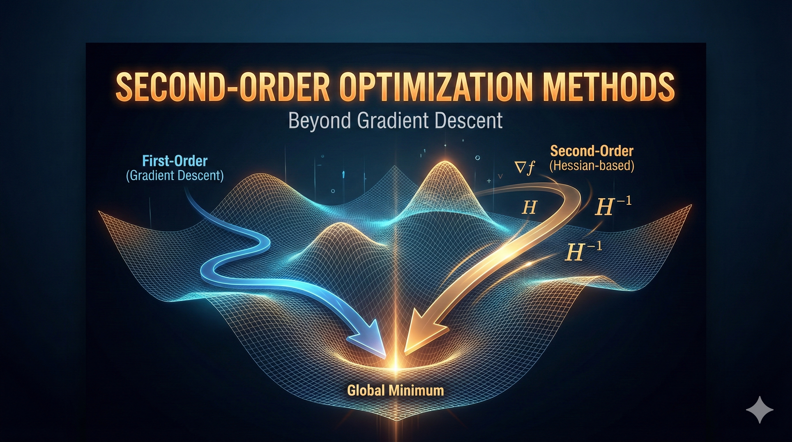
While first-order methods like SGD and Adam dominate deep learning, second-order optimization methods offer powerful alternatives by exploiting curvature information from the loss landscape. In this comprehensive guide, we’ll explore when and how to use these sophisticated techniques.

Key Insight

Second-order methods use the Hessian matrix (second derivatives) to understand the curvature of the loss function, enabling faster convergence with fewer iterations - though at higher computational cost per iteration.

The Limitation of First-Order Methods

Recall that gradient descent uses only the first derivative (gradient):

\[\theta_{t+1} = \theta_t - \alpha \nabla J(\theta_t)\]

This approach has fundamental limitations:

1. No curvature awareness - treats all directions equally
2. Slow convergence in ill-conditioned problems
3. Requires careful learning rate tuning
4. Oscillates in ravines and valleys

graph LR
    A[Optimization Landscape] --> B[First-Order: Gradient Only]
    A --> C[Second-Order: Gradient + Curvature]
    
    B --> D[Slow, Many Iterations]
    C --> E[Fast, Few Iterations]
    
    B --> F[Low Cost Per Iteration]
    C --> G[High Cost Per Iteration]
    
    style B fill:#ff6b6b
    style C fill:#6bcf7f
    style D fill:#ffd93d
    style E fill:#95e1d3

Newton’s Method: The Foundation

Mathematical Formulation

Newton’s method uses a second-order Taylor approximation of the loss function:

\[J(\theta) \approx J(\theta_t) + \nabla J(\theta_t)^T (\theta - \theta_t) + \frac{1}{2}(\theta - \theta_t)^T H(\theta_t) (\theta - \theta_t)\]

Where $H(\theta_t)$ is the Hessian matrix:

\[H_{ij} = \frac{\partial^2 J}{\partial \theta_i \partial \theta_j}\]

Minimizing this quadratic approximation yields the Newton update:

\[\theta_{t+1} = \theta_t - H^{-1}(\theta_t) \nabla J(\theta_t)\]

Intuition: Adaptive Step Sizes

The Hessian inverse $H^{-1}$ acts as an adaptive learning rate matrix:

• Large curvature (steep valley) → small steps
• Small curvature (flat plateau) → large steps
• Negative curvature (saddle point) → direction reversal

This is fundamentally different from first-order methods which use a scalar learning rate!

Python Implementation

import numpy as np
from typing import Callable, Tuple
from scipy.linalg import cho_factor, cho_solve

class NewtonOptimizer:
    """
    Newton's method for unconstrained optimization.
    
    Uses second-order information (Hessian) for faster convergence.
    """
    
    def __init__(
        self,
        damping: float = 1e-4,
        max_iterations: int = 100,
        tolerance: float = 1e-6
    ):
        """
        Args:
            damping: Regularization for Hessian (Levenberg-Marquardt)
            max_iterations: Maximum optimization iterations
            tolerance: Convergence threshold for gradient norm
        """
        self.damping = damping
        self.max_iterations = max_iterations
        self.tolerance = tolerance
        self.history = {'loss': [], 'grad_norm': []}
    
    def optimize(
        self,
        f: Callable,
        grad_f: Callable,
        hess_f: Callable,
        x0: np.ndarray
    ) -> Tuple[np.ndarray, dict]:
        """
        Optimize function using Newton's method.
        
        Args:
            f: Objective function
            grad_f: Gradient function
            hess_f: Hessian function
            x0: Initial parameters
            
        Returns:
            Optimal parameters and optimization history
        """
        x = x0.copy()
        
        for iteration in range(self.max_iterations):
            # Compute gradient and Hessian
            grad = grad_f(x)
            hess = hess_f(x)
            
            # Check convergence
            grad_norm = np.linalg.norm(grad)
            if grad_norm < self.tolerance:
                print(f"Converged at iteration {iteration}")
                break
            
            # Regularize Hessian (Levenberg-Marquardt damping)
            hess_reg = hess + self.damping * np.eye(len(x))
            
            # Solve Newton system: H * delta = -grad
            try:
                # Use Cholesky decomposition for efficiency
                c, low = cho_factor(hess_reg)
                delta = -cho_solve((c, low), grad)
            except np.linalg.LinAlgError:
                # Fallback to regularized inverse
                delta = -np.linalg.solve(
                    hess_reg + 1e-3 * np.eye(len(x)),
                    grad
                )
            
            # Line search (backtracking)
            alpha = self._line_search(f, x, delta, grad)
            
            # Update parameters
            x = x + alpha * delta
            
            # Track progress
            self.history['loss'].append(f(x))
            self.history['grad_norm'].append(grad_norm)
            
            if iteration % 10 == 0:
                print(f"Iter {iteration}: loss={f(x):.6f}, ||grad||={grad_norm:.6f}")
        
        return x, self.history
    
    def _line_search(
        self,
        f: Callable,
        x: np.ndarray,
        direction: np.ndarray,
        grad: np.ndarray,
        alpha_init: float = 1.0,
        rho: float = 0.5,
        c: float = 1e-4
    ) -> float:
        """
        Backtracking line search (Armijo condition).
        
        Args:
            f: Objective function
            x: Current parameters
            direction: Search direction
            grad: Current gradient
            alpha_init: Initial step size
            rho: Backtracking factor
            c: Armijo constant
            
        Returns:
            Step size satisfying Armijo condition
        """
        alpha = alpha_init
        fx = f(x)
        descent = grad.dot(direction)
        
        while f(x + alpha * direction) > fx + c * alpha * descent:
            alpha *= rho
            if alpha < 1e-10:
                break
        
        return alpha


# Example: Rosenbrock function optimization
def rosenbrock(x):
    """Rosenbrock function: f(x,y) = (1-x)^2 + 100(y-x^2)^2"""
    return (1 - x[0])**2 + 100 * (x[1] - x[0]**2)**2

def rosenbrock_grad(x):
    """Gradient of Rosenbrock function."""
    dx = -2*(1 - x[0]) - 400*x[0]*(x[1] - x[0]**2)
    dy = 200*(x[1] - x[0]**2)
    return np.array([dx, dy])

def rosenbrock_hess(x):
    """Hessian of Rosenbrock function."""
    h11 = 2 - 400*(x[1] - x[0]**2) + 800*x[0]**2
    h12 = -400*x[0]
    h22 = 200
    return np.array([[h11, h12], [h12, h22]])

# Run optimization
optimizer = NewtonOptimizer(damping=1e-4)
x_opt, history = optimizer.optimize(
    rosenbrock,
    rosenbrock_grad,
    rosenbrock_hess,
    x0=np.array([-1.0, 1.0])
)

print(f"\nOptimal solution: {x_opt}")
print(f"Optimal value: {rosenbrock(x_opt):.10f}")

The Computational Challenge

Hessian Complexity

For a model with $n$ parameters:

• Gradient: $O(n)$ storage, $O(n)$ computation
• Hessian: $O(n^2)$ storage, $O(n^3)$ inversion

For deep learning models with millions of parameters, this is prohibitively expensive!

Warning: Scalability

A model with 1 million parameters would require ~4 TB to store the Hessian matrix in memory. This makes exact Newton’s method impractical for deep learning.

Quasi-Newton Methods: Practical Alternatives

L-BFGS: Limited-Memory BFGS

L-BFGS (Limited-memory Broyden-Fletcher-Goldfarb-Shanno) approximates the Hessian inverse using only gradient information from recent iterations.

Key Ideas

1. Don’t compute Hessian - approximate $H^{-1}$ implicitly
2. Use gradient history - store only last $m$ gradient pairs
3. Two-loop recursion - efficient computation of search direction

Mathematical Framework

Instead of storing $H^{-1}$, L-BFGS maintains:

\[\begin{aligned} s_k &= \theta_{k+1} - \theta_k \\ y_k &= \nabla J(\theta_{k+1}) - \nabla J(\theta_k) \end{aligned}\]

The Hessian inverse approximation is built recursively:

\[H_k^{-1} = V_k^T H_{k-1}^{-1} V_k + \rho_k s_k s_k^T\]

Where $\rho_k = \frac{1}{y_k^T s_k}$ and $V_k = I - \rho_k y_k s_k^T$

Complete L-BFGS Implementation

from collections import deque

class LBFGSOptimizer:
    """
    L-BFGS optimizer with two-loop recursion.
    
    Memory-efficient quasi-Newton method suitable for large-scale problems.
    """
    
    def __init__(
        self,
        memory_size: int = 10,
        max_iterations: int = 100,
        tolerance: float = 1e-5,
        line_search_max_iter: int = 20
    ):
        """
        Args:
            memory_size: Number of (s, y) pairs to store
            max_iterations: Maximum optimization iterations
            tolerance: Convergence threshold
            line_search_max_iter: Max line search iterations
        """
        self.m = memory_size
        self.max_iterations = max_iterations
        self.tolerance = tolerance
        self.line_search_max_iter = line_search_max_iter
        
        # Storage for gradient differences
        self.s_history = deque(maxlen=memory_size)  # Parameter differences
        self.y_history = deque(maxlen=memory_size)  # Gradient differences
        self.rho_history = deque(maxlen=memory_size)  # 1 / (y^T s)
        
        self.history = {'loss': [], 'grad_norm': []}
    
    def optimize(
        self,
        f: Callable,
        grad_f: Callable,
        x0: np.ndarray
    ) -> Tuple[np.ndarray, dict]:
        """
        Optimize using L-BFGS.
        
        Args:
            f: Objective function
            grad_f: Gradient function
            x0: Initial parameters
            
        Returns:
            Optimal parameters and history
        """
        x = x0.copy()
        grad = grad_f(x)
        
        for iteration in range(self.max_iterations):
            # Check convergence
            grad_norm = np.linalg.norm(grad)
            self.history['grad_norm'].append(grad_norm)
            self.history['loss'].append(f(x))
            
            if grad_norm < self.tolerance:
                print(f"Converged at iteration {iteration}")
                break
            
            # Compute search direction using two-loop recursion
            direction = self._two_loop_recursion(grad)
            
            # Line search
            alpha = self._strong_wolfe_line_search(f, grad_f, x, direction, grad)
            
            # Update parameters
            x_new = x + alpha * direction
            grad_new = grad_f(x_new)
            
            # Update history
            s = x_new - x
            y = grad_new - grad
            
            # Check curvature condition
            sy = s.dot(y)
            if sy > 1e-10:
                self.s_history.append(s)
                self.y_history.append(y)
                self.rho_history.append(1.0 / sy)
            
            x = x_new
            grad = grad_new
            
            if iteration % 10 == 0:
                print(f"Iter {iteration}: loss={f(x):.6f}, ||grad||={grad_norm:.6f}")
        
        return x, self.history
    
    def _two_loop_recursion(self, grad: np.ndarray) -> np.ndarray:
        """
        Compute search direction using L-BFGS two-loop recursion.
        
        This efficiently computes H^{-1} @ grad without forming H^{-1}.
        
        Args:
            grad: Current gradient
            
        Returns:
            Search direction
        """
        q = grad.copy()
        alphas = []
        
        # First loop (backward)
        for s, y, rho in zip(
            reversed(self.s_history),
            reversed(self.y_history),
            reversed(self.rho_history)
        ):
            alpha = rho * s.dot(q)
            q = q - alpha * y
            alphas.append(alpha)
        
        # Initial Hessian approximation (scaling)
        if len(self.s_history) > 0:
            s_last = self.s_history[-1]
            y_last = self.y_history[-1]
            gamma = s_last.dot(y_last) / y_last.dot(y_last)
            r = gamma * q
        else:
            r = q
        
        # Second loop (forward)
        alphas.reverse()
        for s, y, rho, alpha in zip(
            self.s_history,
            self.y_history,
            self.rho_history,
            alphas
        ):
            beta = rho * y.dot(r)
            r = r + s * (alpha - beta)
        
        return -r
    
    def _strong_wolfe_line_search(
        self,
        f: Callable,
        grad_f: Callable,
        x: np.ndarray,
        direction: np.ndarray,
        grad: np.ndarray,
        c1: float = 1e-4,
        c2: float = 0.9
    ) -> float:
        """
        Strong Wolfe line search.
        
        Finds step size satisfying both Armijo and curvature conditions.
        
        Args:
            f: Objective function
            grad_f: Gradient function
            x: Current parameters
            direction: Search direction
            grad: Current gradient
            c1: Armijo constant
            c2: Curvature constant
            
        Returns:
            Step size
        """
        alpha = 1.0
        fx = f(x)
        descent = grad.dot(direction)
        
        # Simple backtracking (simplified Wolfe)
        for _ in range(self.line_search_max_iter):
            x_new = x + alpha * direction
            fx_new = f(x_new)
            
            # Armijo condition
            if fx_new <= fx + c1 * alpha * descent:
                # Curvature condition (simplified)
                grad_new = grad_f(x_new)
                if abs(grad_new.dot(direction)) <= c2 * abs(descent):
                    return alpha
            
            alpha *= 0.5
        
        return alpha


# Example usage
lbfgs = LBFGSOptimizer(memory_size=10)
x_opt, history = lbfgs.optimize(
    rosenbrock,
    rosenbrock_grad,
    x0=np.array([-1.0, 1.0])
)

print(f"\nL-BFGS Optimal solution: {x_opt}")
print(f"L-BFGS Optimal value: {rosenbrock(x_opt):.10f}")

Natural Gradient Descent

The Information Geometry Perspective

Natural Gradient considers the geometry of the parameter space using the Fisher Information Matrix:

\[F(\theta) = \mathbb{E}_{p(x|\theta)} \left[ \nabla \log p(x|\theta) \nabla \log p(x|\theta)^T \right]\]

The natural gradient update is:

\[\theta_{t+1} = \theta_t - \alpha F^{-1}(\theta_t) \nabla J(\theta_t)\]

Why Natural Gradient?

Standard gradient descent is not invariant to reparameterization. Natural gradient uses the Riemannian metric defined by the Fisher matrix, making it invariant to parameter transformations.

class NaturalGradientOptimizer:
    """
    Natural Gradient Descent using Fisher Information Matrix.
    
    Particularly effective for probabilistic models and policy gradient methods.
    """
    
    def __init__(
        self,
        learning_rate: float = 0.01,
        damping: float = 1e-4,
        max_iterations: int = 100
    ):
        self.learning_rate = learning_rate
        self.damping = damping
        self.max_iterations = max_iterations
    
    def compute_fisher_matrix(
        self,
        log_prob_fn: Callable,
        params: np.ndarray,
        samples: np.ndarray
    ) -> np.ndarray:
        """
        Compute Fisher Information Matrix empirically.
        
        Args:
            log_prob_fn: Log probability function
            params: Current parameters
            samples: Data samples
            
        Returns:
            Fisher matrix approximation
        """
        n_params = len(params)
        fisher = np.zeros((n_params, n_params))
        
        for sample in samples:
            # Compute score (gradient of log-likelihood)
            score = self._compute_score(log_prob_fn, params, sample)
            
            # Outer product
            fisher += np.outer(score, score)
        
        fisher /= len(samples)
        return fisher
    
    def _compute_score(
        self,
        log_prob_fn: Callable,
        params: np.ndarray,
        sample: np.ndarray,
        eps: float = 1e-5
    ) -> np.ndarray:
        """Compute score function (gradient of log-prob) numerically."""
        score = np.zeros_like(params)
        
        for i in range(len(params)):
            params_plus = params.copy()
            params_minus = params.copy()
            params_plus[i] += eps
            params_minus[i] -= eps
            
            score[i] = (
                log_prob_fn(params_plus, sample) - 
                log_prob_fn(params_minus, sample)
            ) / (2 * eps)
        
        return score
    
    def update(
        self,
        params: np.ndarray,
        gradient: np.ndarray,
        fisher: np.ndarray
    ) -> np.ndarray:
        """
        Natural gradient update.
        
        Args:
            params: Current parameters
            gradient: Standard gradient
            fisher: Fisher information matrix
            
        Returns:
            Updated parameters
        """
        # Regularize Fisher matrix
        fisher_reg = fisher + self.damping * np.eye(len(params))
        
        # Compute natural gradient
        try:
            natural_grad = np.linalg.solve(fisher_reg, gradient)
        except np.linalg.LinAlgError:
            # Fallback to standard gradient
            natural_grad = gradient
        
        # Update parameters
        params_new = params - self.learning_rate * natural_grad
        
        return params_new

Comparison: When to Use Each Method

graph TD
    A[Choose Optimization Method] --> B{Problem Size?}
    
    B -->|Small n < 1000| C[Newton's Method]
    B -->|Medium 1000 < n < 100k| D[L-BFGS]
    B -->|Large n > 100k| E{Problem Type?}
    
    E -->|Probabilistic Model| F[Natural Gradient]
    E -->|General Deep Learning| G[Adam/SGD]
    
    C --> H[Fast Convergence<br/>Few Iterations]
    D --> I[Good Convergence<br/>Memory Efficient]
    F --> J[Invariant Updates<br/>RL/Bayesian]
    G --> K[Scalable<br/>Stochastic]
    
    style C fill:#6bcf7f
    style D fill:#95e1d3
    style F fill:#ffd93d
    style G fill:#ff6b6b

Decision Matrix

Method	Best For	Pros	Cons	Memory
Newton	Small-scale, convex	Quadratic convergence	$O(n^3)$ cost	$O(n^2)$
L-BFGS	Medium-scale, batch	Fast, memory-efficient	Requires full batch	$O(mn)$
Natural Gradient	Probabilistic models, RL	Parameter-invariant	Fisher computation	$O(n^2)$
Adam	Large-scale, stochastic	Scalable, robust	Slower convergence	$O(n)$

Tip: Hybrid Approaches

Consider using L-BFGS for final fine-tuning after pre-training with Adam. This combines the scalability of first-order methods with the fast convergence of second-order methods.

Practical Applications

1. Logistic Regression with L-BFGS

from scipy.optimize import minimize

def logistic_loss_and_grad(params, X, y):
    """Compute logistic loss and gradient."""
    z = X.dot(params)
    predictions = 1 / (1 + np.exp(-z))
    
    # Loss
    loss = -np.mean(y * np.log(predictions + 1e-10) + 
                    (1 - y) * np.log(1 - predictions + 1e-10))
    
    # Gradient
    grad = X.T.dot(predictions - y) / len(y)
    
    return loss, grad

# Use scipy's L-BFGS implementation
result = minimize(
    fun=lambda w: logistic_loss_and_grad(w, X_train, y_train)[0],
    x0=np.zeros(X_train.shape[1]),
    method='L-BFGS-B',
    jac=lambda w: logistic_loss_and_grad(w, X_train, y_train)[1],
    options={'maxiter': 100, 'disp': True}
)

print(f"Optimal weights: {result.x}")
print(f"Final loss: {result.fun}")

2. Neural Network Fine-Tuning

import torch
import torch.nn as nn

class LBFGSFineTuner:
    """Fine-tune neural network with L-BFGS."""
    
    def __init__(self, model: nn.Module, max_iter: int = 20):
        self.model = model
        self.max_iter = max_iter
    
    def fine_tune(self, train_loader, criterion):
        """Fine-tune model using L-BFGS."""
        optimizer = torch.optim.LBFGS(
            self.model.parameters(),
            lr=1.0,
            max_iter=self.max_iter,
            history_size=10,
            line_search_fn='strong_wolfe'
        )
        
        def closure():
            optimizer.zero_grad()
            total_loss = 0
            
            for inputs, targets in train_loader:
                outputs = self.model(inputs)
                loss = criterion(outputs, targets)
                loss.backward()
                total_loss += loss.item()
            
            return total_loss
        
        optimizer.step(closure)
        
        return self.model

Looking Ahead: Knowledge Graphs

While second-order methods excel at optimization, the next frontier in AI involves structured knowledge representation. In our upcoming series on Knowledge Graphs, we’ll explore:

• How to represent complex relationships between entities
• Graph neural networks for reasoning over structured data
• Combining symbolic knowledge with neural optimization
• Applications in recommendation systems, drug discovery, and NLP

Coming Soon

Our next post will introduce Knowledge Graphs fundamentals - representing the world’s knowledge as interconnected entities and relationships. We’ll show how optimization techniques (including those covered here) apply to learning graph embeddings!

Conclusion

Second-order optimization methods offer powerful tools for specific scenarios:

Key Takeaways

1. Newton’s Method - Quadratic convergence but $O(n^3)$ cost
2. L-BFGS - Practical quasi-Newton for medium-scale problems
3. Natural Gradient - Geometrically principled for probabilistic models
4. Hybrid Strategies - Combine first and second-order methods

When to Use Second-Order Methods

• ✅ Small to medium models (< 100k parameters)
• ✅ Batch optimization (full dataset fits in memory)
• ✅ Fine-tuning pre-trained models
• ✅ Convex or near-convex problems
• ✅ High-precision requirements

When to Stick with First-Order

• ❌ Large-scale deep learning (millions of parameters)
• ❌ Stochastic/mini-batch training
• ❌ Limited memory environments
• ❌ Highly non-convex landscapes

References

1. Nocedal & Wright (2006). “Numerical Optimization” - The definitive reference
2. Martens (2010). “Deep learning via Hessian-free optimization”
3. Amari (1998). “Natural Gradient Works Efficiently in Learning”
4. Liu & Nocedal (1989). “On the Limited Memory BFGS Method”
5. Bottou et al. (2018). “Optimization Methods for Large-Scale Machine Learning”

---

Related Posts:

• Introduction to Gradient Descent
• Momentum and Adaptive Learning Rates
• Knowledge Graphs Fundamentals

---