Agreement Before Accuracy: Auditing the Labels You Are About to Train On
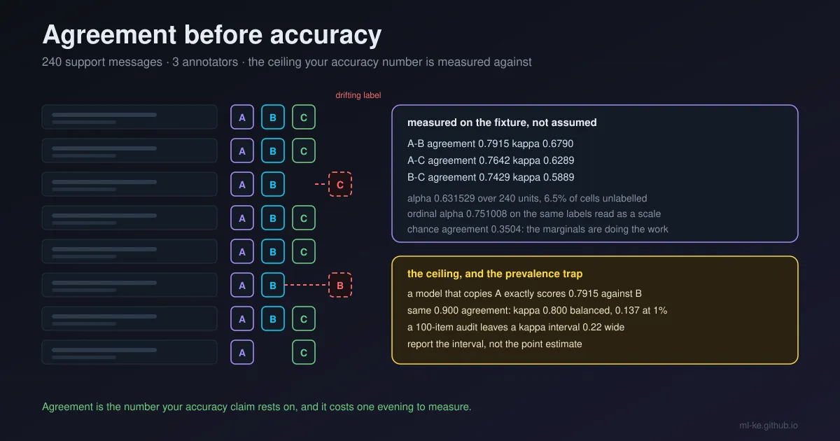
Two numbers from the fixture in this post: three annotators labelling 240 support messages match each other on 74 to 79 percent of the items they both labelled, and an oracle that copies annotator A exactly scores 0.7915 against annotator B. Both come out of standard-library Python below, along with the four coefficients that decide whether your labels are worth training on, and how many items you need before any of those numbers is stable.
Every supervised project pays for labels before it pays for anything else. The labels arrive, someone reports that “the annotators agreed”, and the number turns out to be percent agreement, which is high for a reason that has nothing to do with care: when one class dominates, two annotators who both default to it agree most of the time.
Agreement is the quantity your accuracy metric is measured against. It is also the cheapest thing in the pipeline to compute, and the one most often skipped, so this post builds a single annotation round you can reproduce in an evening and then reads it four ways. The payoff is two decisions that hold up in a review: which coefficient answers the question you are asking, and how wide the interval around it is.
The fixture: 240 messages, three annotators, one bad habit
The task is intent labelling for a mobile-money support desk, the kind of queue where messages arrive in English, Swahili and Sheng mixed together. Four labels: balance, pin, agent, other. Three annotators, A, B and C, with different error rates and one shared habit that turns out to matter more than the error rate: most of their mistakes land in other. That is what a hard queue looks like in practice, because other is a valid answer and the path of least resistance.
The fixture also reproduces two real properties of annotation rounds. Seven percent of cells are missing, as they are when a shift hands over mid-batch, and the second variable is ordinal (severity, 1 to 3) rather than nominal, so the coefficients can be compared on data that has an order.
1
2
3
4
5
6
7
8
9
10
11
12
13
14
15
16
17
18
19
20
21
22
23
24
25
26
27
28
29
30
31
32
33
34
35
36
37
38
39
40
41
42
43
44
45
46
47
48
49
50
51
52
53
54
55
56
57
58
59
60
61
62
63
64
65
66
67
68
69
70
71
72
73
74
75
76
77
78
79
80
81
82
83
84
85
86
87
88
89
90
91
92
93
94
95
96
97
98
99
100
101
102
103
104
105
106
107
108
109
110
111
112
113
114
115
116
117
118
119
120
121
122
123
124
125
126
127
128
129
130
131
132
133
134
135
136
137
138
139
140
141
142
143
144
145
146
147
148
149
150
151
152
153
154
155
156
157
158
159
160
161
162
163
164
import random
from collections import Counter

LABELS = ["other", "balance", "pin", "agent"]
PRIOR = [("other", 0.46), ("balance", 0.24), ("pin", 0.18), ("agent", 0.12)]
PROFILE = {"A": (0.10, 0.55), "B": (0.16, 0.65), "C": (0.22, 0.75)}  # error rate, share dumped into "other"
N_ITEMS, MISSING = 240, 0.07


def draw(rng):
    r, acc = rng.random(), 0.0
    for lab, p in PRIOR:
        acc += p
        if r < acc:
            return lab
    return "other"


def build(seed=7, n_items=N_ITEMS, missing=MISSING):
    rng, units, truth = random.Random(seed), [], []
    for _ in range(n_items):
        t = draw(rng)
        truth.append(t)
        row = {}
        for name, (err, dump) in PROFILE.items():
            if rng.random() < missing:          # shift handover: nobody labelled this one
                row[name] = None
                continue
            if rng.random() < err:
                row[name] = "other" if rng.random() < dump else rng.choice([l for l in LABELS if l != t])
            else:
                row[name] = t
        units.append(row)
    return units, truth


def pct_agree(pairs):
    return sum(1 for a, b in pairs if a == b) / len(pairs)


def cohen_kappa(pairs):
    """Two coders, complete pairs only."""
    po = pct_agree(pairs)
    ca, cb, n = Counter(a for a, _ in pairs), Counter(b for _, b in pairs), len(pairs)
    pe = sum((ca[k] / n) * (cb[k] / n) for k in set(ca) | set(cb))
    return (po - pe) / (1 - pe), po, pe


def fleiss_kappa(units, names, cats):
    """Any number of coders, units where every coder was present."""
    counts = [[sum(1 for n in names if u[n] == c) for c in cats]
              for u in units if all(u[n] is not None for n in names)]
    m, N = len(names), len(counts)
    P = [(sum(c * c for c in row) - m) / (m * (m - 1)) for row in counts]
    pj = [sum(row[j] for row in counts) / (N * m) for j in range(len(cats))]
    pe = sum(p * p for p in pj)
    return (sum(P) / N - pe) / (1 - pe), N


def coincidence(units, names, cats, metric):
    """Krippendorff's coincidence matrix -> (observed, expected) disagreement.

    Marginals are counted over pairable units only, which matters for ordinal data.
    """
    val = {c: i for i, c in enumerate(cats)}
    V = len(cats)
    o = [[0.0] * V for _ in range(V)]
    counts = [0] * V
    n = 0.0
    for u in units:
        present = [u[k] for k in names if u[k] is not None]
        m = len(present)
        if m < 2:                               # a single rating is not pairable
            continue
        n += m
        for a in range(m):
            counts[val[present[a]]] += 1
            for b in range(m):
                if a != b:
                    o[val[present[a]]][val[present[b]]] += 1.0 / (m - 1)
    nc = [sum(o[i]) for i in range(V)]
    Do = sum(o[c][k] * metric(cats[c], cats[k], counts) for c in range(V) for k in range(V)) / n
    De = sum(nc[c] * nc[k] * metric(cats[c], cats[k], counts)
             for c in range(V) for k in range(V)) / (n * (n - 1))
    return Do, De


def alpha(units, names, cats, metric=lambda a, b, counts: 0.0 if a == b else 1.0):
    Do, De = coincidence(units, names, cats, metric)
    return 1 - Do / De


names = ["A", "B", "C"]
units, truth = build()
cells = len(units) * len(names)
print(f"items {len(units)}  annotators {len(names)}  cells {cells}  "
      f"cells missing {sum(1 for u in units for k in names if u[k] is None) / cells:.1%}")
for i, x in enumerate(names):
    for y in names[i + 1:]:
        pairs = [(u[x], u[y]) for u in units if u[x] is not None and u[y] is not None]
        k, po, pe = cohen_kappa(pairs)
        print(f"  {x}-{y}  n={len(pairs)}  agree {po:.4f}  chance {pe:.4f}  kappa {k:+.4f}"
              f"   copy {x} scored against {y}: {po:.4f}")
fk, Nu = fleiss_kappa(units, names, LABELS)
comp = [u for u in units if all(u[k] is not None for k in names)]
print(f"Fleiss kappa, {Nu} complete units        : {fk:.6f}")
print(f"alpha nominal, every unit (missing kept): {alpha(units, names, LABELS):.6f}")
print(f"alpha nominal, complete units only      : {alpha(comp, names, LABELS):.6f}")
print(f"difference on the same units            : {alpha(comp, names, LABELS) - fk:+.2e}")
print("accuracy against the fixture's latent truth: " +
      "  ".join(f"{x} {sum(1 for u, t in zip(units, truth) if u[x] == t) / len(units):.3f}" for x in names))

# same 240 items, second variable: severity 1 mild .. 3 urgent, coders move one step
SEV_PRIOR = [(1, 0.50), (2, 0.35), (3, 0.15)]
SEV_ERR = {"A": 0.12, "B": 0.18, "C": 0.24}


def build_severity(seed=11, n_items=N_ITEMS, missing=MISSING):
    rng, rows = random.Random(seed), []
    for _ in range(n_items):
        r, acc = rng.random(), 0.0
        for v, p in SEV_PRIOR:
            acc += p
            if r < acc:
                true_v = v
                break
        row = {}
        for name, err in SEV_ERR.items():
            if rng.random() < missing:
                row[name] = None
                continue
            v = true_v if rng.random() >= err else min(3, max(1, true_v + rng.choice([-1, 1])))
            row[name] = v
        rows.append(row)
    return rows


sev = build_severity()
svals = sorted({v for d in sev for v in d.values() if v is not None})


def ordinal_metric(a, b, counts):
    """Krippendorff's ordinal difference: pairable values between the two categories,
    minus half the two end categories, squared."""
    i, j = svals.index(a), svals.index(b)
    if i == j:
        return 0.0
    lo, hi = min(i, j), max(i, j)
    between = sum(counts[r] for r in range(lo, hi + 1))
    return (between - (counts[i] + counts[j]) / 2) ** 2


print(f"alpha ordinal on the 1-3 severity scale : {alpha(sev, names, svals, ordinal_metric):.6f}")
print(f"alpha nominal on the same severity scale: {alpha(sev, names, svals):.6f}")

print()
print("the alpha-minus-Fleiss gap on complete units, as the sample grows (same generator, longer runs)")
for n_items in (240, 2400, 24000):
    u, _ = build(n_items=n_items)
    fk_n, Nu_n = fleiss_kappa(u, names, LABELS)
    c_n = [x for x in u if all(x[k] is not None for k in names)]
    a_n = alpha(c_n, names, LABELS)
    print(f"  {n_items:>6} items  {Nu_n:>6} complete units   Fleiss {fk_n:.6f}   alpha {a_n:.6f}"
          f"   gap {a_n - fk_n:+.2e}")
1
2
3
4
5
6
7
8
9
10
11
12
13
14
15
16
items 240  annotators 3  cells 720  cells missing 6.5%
  A-B  n=211  agree 0.7915  chance 0.3504  kappa +0.6790   copy A scored against B: 0.7915
  A-C  n=212  agree 0.7642  chance 0.3645  kappa +0.6289   copy A scored against C: 0.7642
  B-C  n=210  agree 0.7429  chance 0.3745  kappa +0.5889   copy B scored against C: 0.7429
Fleiss kappa, 200 complete units        : 0.634913
alpha nominal, every unit (missing kept): 0.631529
alpha nominal, complete units only      : 0.635521
difference on the same units            : +6.08e-04
accuracy against the fixture's latent truth: A 0.858  B 0.783  C 0.787
alpha ordinal on the 1-3 severity scale : 0.751008
alpha nominal on the same severity scale: 0.594901

the alpha-minus-Fleiss gap on complete units, as the sample grows (same generator, longer runs)
     240 items     200 complete units   Fleiss 0.634913   alpha 0.635521   gap +6.08e-04
    2400 items    1964 complete units   Fleiss 0.684523   alpha 0.684577   gap +5.35e-05
   24000 items   19349 complete units   Fleiss 0.699629   alpha 0.699634   gap +5.17e-06
Four numbers on one table, and what each one hides
The line to read first is the one the code prints almost as an aside. A model that copies annotator A reproduces A’s labels perfectly, and when it is scored against annotator B it gets 0.7915, which is exactly the A-B agreement rate. That copy-an-A result needs no theorem to explain it. It is the arithmetic of what a “human-level” target means when the two humans who produced the targets disagree on one item in five. Quote a ceiling with the pair it belongs to: 0.79 for A against B, 0.74 for B against C.
The chance-corrected coefficients in the same block answer a different question, so they need the label distribution next to them. Cohen’s kappa is the two-coder version:
\[\kappa = \frac{p_o - p_e}{1 - p_e}, \qquad p_e = \sum_k p_{k1}\,p_{k2}\]where $p_o$ is observed agreement and $p_e$ is the agreement you would get from the marginals alone. Krippendorff’s alpha replaces the marginals with a coincidence matrix so it can take more than two coders, missing cells and any measurement level:
\[\alpha = 1 - \frac{D_o}{D_e}, \qquad D_o = \frac{1}{n}\sum_{c,k} o_{ck}\,\delta^2_{ck}, \qquad D_e = \frac{1}{n(n-1)}\sum_{c,k} n_c n_k \,\delta^2_{ck}\]On this fixture, Fleiss’ kappa over the 200 fully labelled units is 0.634913 and alpha over all 240 units is 0.631529. The two agree for a structural reason: with the same number of coders per unit and no missing data, nominal alpha and Fleiss’ kappa differ only in the finite-sample correction inside $D_e$, where alpha uses $n_c(n_c-1)$ and Fleiss uses the plug-in marginal squares. The loop at the bottom of the block measures the gap on the same complete units at three sample sizes: $+6.08\times10^{-4}$ at 240 items, $5.35\times10^{-5}$ at 2,400 and $5.17\times10^{-6}$ at 24,000, shrinking by roughly a factor of ten each time the sample grows tenfold. The metric survey states the two-rater case plainly: for nominal data with no missing values, alpha is mathematically equivalent to Cohen’s kappa.
The ordinal line is the one to be careful with. Severity read with the nominally-defined difference function scores 0.594901, and the same data read with the ordinal difference function scores 0.751008. Both are correct. The nominal version treats a one-step miss (mild read as moderate) as identical to a two-step miss (mild read as urgent), which is rarely what a severity reviewer means, and the ordinal version weights by the number of pairable values sitting between the two categories. So when the scale has an order, the measurement level is part of the result, and two papers quoting “alpha 0.59” and “alpha 0.75” on severity data are not disagreeing.
The first trap: accuracy is not agreement
Read the last line of the fixture output next to the first. Annotator A is the most accurate against the hidden truth at 0.858, and it still disagrees with C on 24 of every 100 items the two of them both labelled. B is the least accurate at 0.783 and its disagreement with C, at 0.7429, is the widest of the three pairs. Accuracy against a truth and agreement with a colleague are different properties, and only agreement is observable while the labels are being made, because nobody has the truth yet. Reliability studies measure agreement and argue about validity separately.
The published literature is a warning about how far agreement travels. MasakhaNER, the named-entity corpus for ten African languages, reports Fleiss’ kappa of 0.987 to 1.000 at token level and 0.959 to 1.000 at entity level, with four languages at a perfect 1.000. The method section explains where the perfect scores come from: for those languages two annotators labelled each token and were “instructed to discuss and resolve conflicts among themselves”. That is a legitimate and probably better process, and the number it produces is a statement about the process, not about how reliably two independent annotators would label the text. Before borrowing a reliability number from a paper, read what the annotators were allowed to do.
At the other end, the LAW-XIX 2025 study of emotion annotation sums up the field’s other failure mode: kappa results “ranging from 0.19 to 0.33” for emotion and valence, with weighted alpha from 0.22 to 0.64 on the same data. Low agreement on a subjective task is a finding, not a bug, and it should reach the paper rather than disappear into an average.
The second trap: the same 0.90 agreement, five different kappas
Percent agreement has one moving part, and it is the prevalence of whatever you are counting. The next block holds observed agreement exactly constant at 0.900 and moves only the prevalence of the rare class, which is enough to push kappa from 0.800 to 0.137 without changing how often the two coders matched.
1
2
3
4
5
6
7
8
9
10
11
12
13
14
15
16
17
18
19
20
21
22
23
24
25
26
27
28
29
"""Prevalence sweep: hold observed agreement at 0.900, move the prevalence, watch the chance-corrected
coefficients move. Two coders, two categories, so the arithmetic is exact rather than simulated."""

PO = 0.900
Q = 0.0527864          # each coder's flip rate, from PO = 1 - 2q + 2q^2
PABAK = 2 * PO - 1

print(f"two coders, each mislabelling at rate {Q:.4f} (this is what pins observed agreement at {PO:.3f})")
print("  prevalence   chance Pe    kappa    PABAK      AC1")
for pi in (0.01, 0.02, 0.05, 0.10, 0.25, 0.50):
    p = pi * (1 - Q) + (1 - pi) * Q            # each coder's positive rate
    pe_kappa = p * p + (1 - p) * (1 - p)
    pe_ac1 = 2 * p * (1 - p)                   # Gwet caps chance agreement at 0.5
    print(f"  {pi:>10.1%}   {pe_kappa:>8.4f}   {(PO - pe_kappa) / (1 - pe_kappa):>6.3f}"
          f"   {PABAK:>6.3f}   {(PO - pe_ac1) / (1 - pe_ac1):>6.3f}")

print()
print("one counted 2x2 table instead of a simulated one: a=1 b=0 / c=9 d=230, n=240")
a, b, c, d = 1, 0, 9, 230
n = a + b + c + d
po = (a + d) / n
p1, p2 = (a + b) / n, (a + c) / n
pe_k = p1 * p2 + (1 - p1) * (1 - p2)
pbar = (p1 + p2) / 2
pe_g = 2 * pbar * (1 - pbar)
print(f"  observed agreement {po:.4f}   kappa {(po - pe_k) / (1 - pe_k):+.3f}"
      f"   PABAK {2 * po - 1:.3f}   AC1 {(po - pe_g) / (1 - pe_g):.3f}")
print(f"  specific agreement on the rare label 2a/(2a+b+c) = {2 * a / (2 * a + b + c):.3f}"
      f"   on the common label 2d/(2d+b+c) = {2 * d / (2 * d + b + c):.3f}")
1
2
3
4
5
6
7
8
9
10
11
12
two coders, each mislabelling at rate 0.0528 (this is what pins observed agreement at 0.900)
  prevalence   chance Pe    kappa    PABAK      AC1
        1.0%     0.8842    0.137    0.800    0.887
        2.0%     0.8686    0.239    0.800    0.885
        5.0%     0.8240    0.432    0.800    0.879
       10.0%     0.7560    0.590    0.800    0.868
       25.0%     0.6000    0.750    0.800    0.833
       50.0%     0.5000    0.800    0.800    0.800

one counted 2x2 table instead of a simulated one: a=1 b=0 / c=9 d=230, n=240
  observed agreement 0.9625   kappa +0.176   PABAK 0.925   AC1 0.961
  specific agreement on the rare label 2a/(2a+b+c) = 0.182   on the common label 2d/(2d+b+c) = 0.981
That behaviour is the best-documented complaint about kappa. Feinstein and Cicchetti named two paradoxes: a low kappa can occur at a high agreement, and unbalanced marginals produce higher kappa than balanced ones. The same review records Ludbrook’s judgement on the Landis and Koch bands that most teams quote: the approach “has no sound theoretical basis and can be positively misleading to investigators”. The alternative coefficients in the table are not free of problems either. PABAK, the prevalence-adjusted bias-adjusted kappa, is constant 0.800 here by construction, because it discards the marginals entirely and reports $2p_o - 1$; Gwet’s AC1 barely moves (0.887 to 0.800) because its chance agreement is capped below 0.5. Delgado and Tibau go further and argue that kappa should be avoided as a classification metric altogether, even in the two-class case.
The counted 2x2 table at the bottom of the block is the version of that argument with real cells in it, and it says what to do instead. One item in ten of the rare class is labelled positive by the two coders, and they agree on one of those ten. Observed agreement is 0.9625, kappa is 0.176, PABAK is 0.925, AC1 is 0.961 and the specific agreement on the rare label, $2a/(2a+b+c)$, is 0.182. Four coefficients, four readings of one table. If the rare class is the thing you care about, the aggregate number is mostly a statement about the common class, and the pair of specific agreements (0.182 and 0.981 here) is the one to report.
How many items before the number means something
Every number above is a point estimate from one draw of items. Resample the items and the estimate moves, and the size of the move decides whether the number is reportable at all.
1
2
3
4
5
6
7
8
9
10
11
12
13
14
15
16
17
18
19
20
21
22
23
24
25
26
27
28
29
30
31
32
33
34
35
36
37
38
39
40
41
42
43
44
45
46
47
48
49
50
51
52
53
54
55
56
57
58
59
60
61
62
63
64
65
66
67
68
69
70
71
72
73
74
75
76
"""How wide is the interval around one agreement number? Bootstrap over items, two fixtures:
two coders (Cohen's kappa and percent agreement) and three coders (Krippendorff's alpha)."""
import random
from collections import Counter

LABELS = ["other", "balance", "pin", "agent"]
PRIOR = [("other", 0.46), ("balance", 0.24), ("pin", 0.18), ("agent", 0.12)]
PROFILE = {"A": (0.10, 0.55), "B": (0.16, 0.65), "C": (0.22, 0.75)}


def draw(rng):
    r, acc = rng.random(), 0.0
    for lab, p in PRIOR:
        acc += p
        if r < acc:
            return lab
    return "other"


def synth(n, seed, coders):
    rng, rows = random.Random(seed), []
    for _ in range(n):
        t = draw(rng)
        row = []
        for name in coders:
            err, dump = PROFILE[name]
            if rng.random() < err:
                row.append("other" if rng.random() < dump else rng.choice([l for l in LABELS if l != t]))
            else:
                row.append(t)
        rows.append(tuple(row))
    return rows


def kappa2(rows):
    po = sum(1 for a, b in rows if a == b) / len(rows)
    ca, cb, n = Counter(x for x, _ in rows), Counter(y for _, y in rows), len(rows)
    pe = sum((ca[k] / n) * (cb[k] / n) for k in set(ca) | set(cb))
    return (po - pe) / (1 - pe), po


def alpha3(rows):
    """Nominal Krippendorff's alpha over three coders, coincidence-matrix form."""
    val = {c: i for i, c in enumerate(LABELS)}
    V = len(LABELS)
    o = [[0.0] * V for _ in range(V)]
    n = 0
    for r in rows:
        m = len(r)
        n += m
        for i in range(m):
            for j in range(m):
                if i != j:
                    o[val[r[i]]][val[r[j]]] += 1.0 / (m - 1)
    nc = [sum(o[i]) for i in range(V)]
    Do = sum(o[c][k] for c in range(V) for k in range(V) if c != k) / n
    De = sum(nc[c] * nc[k] for c in range(V) for k in range(V) if c != k) / (n * (n - 1))
    return 1 - Do / De


for n in (50, 100, 200, 400, 800, 2000):
    two = synth(n, n, ("A", "B"))
    three = synth(n, n + 5000, ("A", "B", "C"))
    k0, po0 = kappa2(two)
    a0 = alpha3(three)
    ks, as_ = [], []
    for rep in range(2000):
        r = random.Random(100_000 + rep)
        idx = [r.randrange(n) for _ in range(n)]
        ks.append(kappa2([two[i] for i in idx])[0])
        as_.append(alpha3([three[i] for i in idx]))
    ks.sort()
    as_.sort()
    print(f"  n={n:>4}  agreement {po0:.3f}   kappa {k0:+.3f} CI [{ks[49]:+.3f},{ks[1949]:+.3f}]"
          f" width {ks[1949] - ks[49]:.3f}   alpha {a0:+.3f} CI [{as_[49]:+.3f},{as_[1949]:+.3f}]"
          f" width {as_[1949] - as_[49]:.3f}")
1
2
3
4
5
6
  n=  50  agreement 0.840   kappa +0.766 CI [+0.601,+0.909] width 0.308   alpha +0.599 CI [+0.459,+0.729] width 0.270
  n= 100  agreement 0.820   kappa +0.736 CI [+0.618,+0.840] width 0.223   alpha +0.780 CI [+0.698,+0.856] width 0.158
  n= 200  agreement 0.890   kappa +0.834 CI [+0.762,+0.895] width 0.133   alpha +0.697 CI [+0.622,+0.760] width 0.138
  n= 400  agreement 0.830   kappa +0.747 CI [+0.691,+0.800] width 0.109   alpha +0.651 CI [+0.602,+0.696] width 0.093
  n= 800  agreement 0.835   kappa +0.750 CI [+0.713,+0.788] width 0.074   alpha +0.687 CI [+0.653,+0.718] width 0.065
  n=2000  agreement 0.815   kappa +0.720 CI [+0.694,+0.745] width 0.051   alpha +0.710 CI [+0.690,+0.730] width 0.041
The widths are the useful part. A 100-item reliability sample gives a kappa interval about 0.22 wide, so “our annotators agreed, kappa 0.74” describes anything from 0.62 to 0.84, which spans both a tentative and a comfortable band under any published threshold. Four hundred items halve that, and 2,000 items give roughly plus or minus 0.025. The percentile spread also does not keep pace with the point estimate: at n=200 the kappa point estimate is 0.834 and its interval is 0.133 wide, while at n=400 the point estimate is 0.747 with an interval of 0.109. Comparisons between annotation rounds with a few hundred items each are inside the noise of both intervals.
That is why the metric survey lists interval reporting as guidance rather than etiquette: “point estimates without uncertainty overstate precision and reduce comparability”, with the accompanying recommendation to describe the rater design and account for missing data and label prevalence. The same paper is careful about what a reliability number cannot settle, noting that model-based evaluation can match or exceed human reliability on several text-quality dimensions, so human labels “can no longer serve as an unquestioned gold standard”. Agreement tells you how reproducible the labels are. It does not tell you that they are the right labels for the task.
How to apply this to your own annotation round
| Step | What to record | Why it matters here |
|---|---|---|
| Label a reliability sample independently, without discussion | 100 to 400 items, double-labelled, disagreement not resolved | Consensus procedures produce high agreement by design: MasakhaNER reached kappa 1.000 that way, which measures the process |
| Print the full agreement table, not one number | The 2x2 or k-by-k counts, the label distribution, cells missing | The counted 2x2 above reads as 0.9625 agreement, kappa 0.176, PABAK 0.925 and AC1 0.961 |
| Choose the coefficient from the question | Percent agreement for raw match, kappa for two coders, alpha for many coders or missing cells | The same severity data scored 0.594901 nominal and 0.751008 ordinal |
| Match the difference function to the scale | Ordinal metric for ordered scales, nominal for category sets | Treating a one-step miss as equal to a two-step miss is a modelling decision, not a default |
| Report an interval with the point estimate | Bootstrap over items, 2,000 resamples, percentile bounds | A 100-item audit has a kappa interval about 0.22 wide |
| Set the reliability threshold before training | Krippendorff’s convention: rely on data at 0.800, tentative to 0.667, discard below | Thresholds are conventions, so agree the number while the codebook can still be rewritten |
| Quote a ceiling with the pair it belongs to | The annotator-to-annotator agreement your model is being compared against | An exact copy of A scores 0.7915 against B on this fixture |
| Keep the raw table in the repo | The counts, the seed, the script | Every number in this post is reproducible from the three blocks with no dependencies |
Two implementation notes for the day you wire this into a pipeline. First, the reference implementation expects its reliability matrix as coders by units; feeding the fixture in the other orientation returned $-0.0021$ on data whose alpha is 0.63, which is the kind of number that gets published by accident. Second, the ordinal distance function takes its marginals from pairable units only. Counting every labelled value instead, including items a single coder rated, moved alpha by $1.4\times10^{-5}$ here, which is small enough to look like rounding and large enough to be a different implementation.
Key takeaways
| Question | Answer from this post |
|---|---|
| What is the ceiling on a model’s measured accuracy? | The agreement between the human labels it is scored against: a copy of A scores 0.7915 against B |
| Why did two annotators agree 90 percent of the time and score kappa 0.137? | Chance agreement was 0.8842; the same 0.900 agreement is kappa 0.800 at balanced prevalence |
| Which coefficient should I report? | Percent agreement plus one chance-corrected coefficient, with the label distribution: four coefficients on one 2x2 table read 0.9625, 0.176, 0.925 and 0.961 |
| Does the measurement level change alpha? | Yes. The severity scale scored 0.594901 nominal and 0.751008 ordinal on identical labels |
| How many items do I need? | 100 gives a kappa interval about 0.22 wide, 400 about 0.11, 2,000 about 0.05 |
| Is alpha just Fleiss’ kappa? | On complete units with equal coder counts they differ only by the finite-sample correction: $6.08\times10^{-4}$ at 240 items, $5.17\times10^{-6}$ at 24,000 |
| What does agreement not tell me? | Whether the labels are valid for the task. Reliability is about reproducibility, and models now sometimes match human reliability on structured tasks |
The three blocks are standard-library Python, they print only deterministic output, and every figure quoted above came out of them as published. Pointing them at real data means replacing the fixture with your own labelled sample and keeping the metrics; the coefficients care about the counts, not about the language the messages are in. If you run one thing this week, run the pairwise table with the “copy A scored against B” line next to it, because that is the number your accuracy claim is quietly resting on.
References
- Krippendorff’s reliability bands as summarised in K-Alpha Calculator — alpha at or above 0.800 for reliable conclusions, 0.667 to 0.800 for tentative ones, below 0.667 taken as unreliable
- McHugh, M. L. (2012). Interrater reliability: the kappa statistic, Biochem Med 22(3):276-282 — the kappa bands, and the advice to calculate both percent agreement and kappa
- Xie, Q. (2013). Agree or Disagree? A Demonstration of An Alternative Statistic to Cohen’s Kappa — the Feinstein and Cicchetti paradoxes, Ludbrook on the Landis and Koch bands, Zhao’s twelve additional paradoxes, Gwet’s AC1 chance agreement capped below 0.5
- Delgado, R., Tibau, X-A. (2019). Why Cohen’s Kappa should be avoided as performance measure in classification, PLOS ONE — the prevalence and bias paradoxes, PABAK, and the case against a single coefficient
- Counting on Consensus: Selecting the Right Inter-annotator Agreement Metric for NLP Annotation and Evaluation (2026) — metric selection by data type, interval reporting guidance, and the limits of human labels as a gold standard
- Another Approach to Agreement Measurement and Prediction, LAW-XIX 2025 — kappa 0.19 to 0.33 and weighted alpha 0.22 to 0.64 on emotion and valence annotation
- Adelani, D. I. et al. (2021). MasakhaNER: Named Entity Recognition for African Languages, TACL — Table 4 token- and entity-level Fleiss’ kappa for ten languages, and the conflict-resolution procedure behind the perfect scores
- krippendorff 0.9.0 — the reference alpha implementation this post’s nominal and ordinal values were checked against, equal to twelve decimal places
Related posts
- The Denominator Is the Metric — the same discipline applied to retrieval: know what was counted before you quote a score
- Your Corpus Is Duplicating Itself — measuring corpus hygiene with a filter you can audit
- Split Before You Believe — another evaluation number that dissolves once you check how it was produced
- Evaluating LLMs: Benchmarks That Matter for African Use Cases — why imported scores need a local reference set