Split Before You Believe: Why Offline Fraud Models Score Better Than They Perform

A fraud label does not exist on the day of the transaction

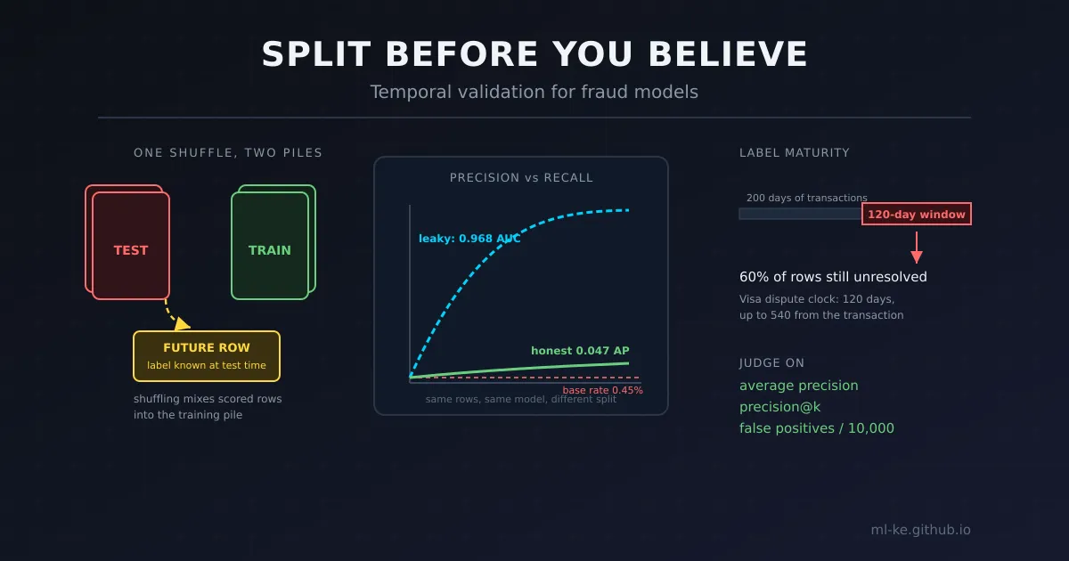
Visa’s dispute rules let an issuer raise a merchandise-not-received dispute “no later than 120 calendar days from the last date the cardholder expected to receive the merchandise or services, not to exceed 540 calendar days from the transaction processing date.” A transaction your model scored on 3 January can be relabelled fraudulent in May, and in some conditions not until the following year. The Central Bank of Kenya’s complaints guidance gives institutions 48 hours to acknowledge a customer complaint and 7 days to resolve it, so the trail that becomes your label moves on a clock measured in weeks.

That one fact breaks the default habit of evaluation. Shuffle a payments dataset, split it 70/30, and you have trained on rows whose outcomes were unknown when the test rows were scored. Kapoor and Narayanan surveyed this failure across research communities and found it in 17 fields, “collectively affecting 329 papers and in some cases leading to wildly overoptimistic conclusions.” Their reproducibility study is blunter: every paper claiming complex ML models beat logistic regression at civil war prediction failed to reproduce because of data leakage.

The framing This post covers the layer before deployment: validating an offline fraud model without lying to yourself. It is not population drift after launch (Fraud Model Drift Monitoring), per-line anomaly detection (Anomaly Detection for Reconciliation), the generic drift taxonomy (ML Monitoring), feature selection (Fraud ML in Mobile Money), or the transaction graph (Graph Fraud Ring Detection). Those assume the reported number was honest; this one is about earning it.

Random splits borrow information that did not exist yet

Kaufman, Rosset, Perlich and Stitelman define the failure precisely in ACM TKDD: leakage is “the introduction of information about the data mining target that should not be legitimately available to mine from.” In a fraud pipeline it is usually not a stray column but a sequence:

1. Build account-level history features over the full table, including rows from the scoring period.
2. Shuffle and split.
3. Fit and evaluate.

Step 1 makes step 2 fatal. An aggregate such as “share of this account’s transactions that were fraud” spans the whole table, including rows the model will be tested on.

Temporal drift compounds it. Fraud is not stationary: an account behaves normally for months, runs a burst, then goes quiet. Rows close together in time are alike, so a shuffled split grades the model on the regime it just memorised. Google’s Rule #33 gives the honest alternative: “If you produce a model based on the data until January 5th, test the model on the data from January 6th and after.”

The demo: one model, two splits

The script below builds 24,000 KES transactions over 200 days with random.seed(20260917), so the output is reproducible. Three percent of accounts drift into a compromise window; the rest never do. Each row carries a day index, a night flag, a log amount and a label driven by a latent per-account state the model never sees.

One account-history feature is computed two ways: r[5] uses only that account’s earlier rows, which is what a scoring job actually has, while r[6] is the account’s fraud rate over the whole table, possible only if features are built before splitting. The same logistic regression is fit and scored under a shuffled 70/30 split and a time-ordered split at day 140.

import random, math

SEED, DAYS, N, N_ACCT, HOLD = 20260917, 200, 24000, 600, 120
random.seed(SEED)
sig = lambda z: 1.0 / (1.0 + math.exp(-z))

# 1. Accounts: 3% drift into a compromise window - hot in one period, quiet in the next.
acc = []
for _ in range(N_ACCT):
    if random.random() < 0.03:
        on = random.randrange(0, DAYS)
        acc.append({"risk": random.gauss(0, 1), "on": on, "off": on + random.randrange(15, 60)})
    else:
        acc.append({"risk": random.gauss(0, 1), "on": -1, "off": -1})

# 2. Transactions, timestamped in day order. `hot` is the latent truth the model never sees.
rows = []
for i in range(N):
    d, a = int(DAYS * i / N), random.randrange(N_ACCT)
    night, amt = int(random.random() < 0.18), math.exp(random.gauss(0, 1.1))
    A = acc[a]
    hot = 1.0 if A["on"] <= d < A["off"] else 0.0
    p = sig(-7.4 + 8.0 * hot + 0.7 * A["risk"] + 0.9 * night + 0.4 * math.log(amt))
    rows.append([a, d, night, math.log(amt) / 1.1, int(random.random() < p)])

# 3. One account-history feature, two ways: r[5] uses past rows only, r[6] the whole dataset.
tot, hit, seen, prior = {}, {}, {}, {}
for r in rows:
    tot[r[0]] = tot.get(r[0], 0) + 1
    hit[r[0]] = hit.get(r[0], 0) + r[4]
for r in rows:
    a = r[0]
    r.append(min((seen.get(a, 0) + 0.0024) / (prior.get(a, 0) + 0.4), 0.6))
    r.append(min(hit[a] / tot[a], 0.6))
    seen[a], prior[a] = seen.get(a, 0) + r[4], prior.get(a, 0) + 1

# 4. Logistic regression by plain gradient descent; features standardised.
def fit(tr, j):
    y = [r[4] for r in tr]
    F = [(r[2], r[3], r[j]) for r in tr]
    mu = [sum(c[k] for c in F) / len(F) for k in range(3)]
    sd = [max((sum(c[k] ** 2 for c in F) / len(F) - mu[k] ** 2) ** 0.5, 1e-6) for k in range(3)]
    X = [tuple((c[k] - mu[k]) / sd[k] for k in range(3)) for c in F]
    w = [0.0] * 4
    for _ in range(400):
        g = [0.0] * 4
        for (x1, x2, x3), t in zip(X, y):
            e = sig(w[0] + w[1] * x1 + w[2] * x2 + w[3] * x3) - t
            g[0] += e; g[1] += e * x1; g[2] += e * x2; g[3] += e * x3
        w = [a - b / len(X) for a, b in zip(w, g)]
    return w, mu, sd

def score(te, w, mu, sd, j):
    return [sig(w[0] + w[1] * (r[2] - mu[0]) / sd[0] + w[2] * (r[3] - mu[1]) / sd[1]
                + w[3] * (r[j] - mu[2]) / sd[2]) for r in te]

def auc(s, y):                                    # rank formula, tied scores averaged
    p, rk, i = sorted(zip(s, y)), [0.0] * len(s), 0
    while i < len(p):
        j = i
        while j + 1 < len(p) and p[j + 1][0] == p[i][0]: j += 1
        for k in range(i, j + 1): rk[k] = (i + j) / 2.0 + 1.0
        i = j + 1
    P, Nn = sum(y), len(y) - sum(y)
    return (sum(rk[k] for k in range(len(p)) if p[k][1]) - P * (P + 1) / 2.0) / (P * Nn)

def ap(s, y):                                     # step average precision
    tp, tot = 0, 0.0
    for k, i in enumerate(sorted(range(len(s)), key=lambda i: -s[i]), 1):
        if y[i]: tp += 1; tot += tp / k
    return tot / sum(y)

# 5. Same rows, same model, two splits.
ri = list(range(len(rows))); random.shuffle(ri); cut = int(0.7 * len(rows))
runs = (("random split       + full-history feature", [rows[i] for i in ri[:cut]], [rows[i] for i in ri[cut:]], 6),
        ("time-ordered split + point-in-time feature", [r for r in rows if r[1] < 140], [r for r in rows if r[1] >= 140], 5))
print(f"rows={len(rows)}  prevalence={sum(r[4] for r in rows)/len(rows):.4f}  seed={SEED}")
out = []
for name, tr, te, j in runs:
    w, mu, sd = fit(tr, j)
    s, y = score(te, w, mu, sd, j), [r[4] for r in te]
    out.append((auc(s, y), ap(s, y)))
    print(f"{name}: train={len(tr)} test={len(te)} pos={sum(y)} ROC-AUC={out[-1][0]:.3f}  avg-precision={out[-1][1]:.3f}")
print(f"gap: ROC-AUC {out[0][0]-out[1][0]:.3f}   avg-precision {out[0][1]-out[1][1]:.3f}")
pend = sum(1 for r in rows if r[1] >= DAYS - HOLD)
print(f"unresolved labels with a {HOLD}-day confirmation window: {pend}/{len(rows)} = {pend/len(rows):.0%} of rows")

Run it with python3 demo.py:

rows=24000  prevalence=0.0045  seed=20260917
random split       + full-history feature: train=16800 test=7200 pos=38 ROC-AUC=0.968  avg-precision=0.279
time-ordered split + point-in-time feature: train=16800 test=7200 pos=36 ROC-AUC=0.789  avg-precision=0.047
gap: ROC-AUC 0.179   avg-precision 0.232
unresolved labels with a 120-day confirmation window: 14400/24000 = 60% of rows

Both pipelines see 16,800 training rows and 7,200 test rows, with 38 and 36 positives, so the difference is the split rather than the sample size. Prevalence is 0.45%.

Why ROC-AUC flatters and average precision exposes

ROC-AUC falls from 0.968 to 0.789, a loss of 0.179, and 0.789 is a number most teams would still call good. Average precision falls from 0.279 to 0.047, a loss of 0.232, roughly a sixfold collapse. The metric that flatters the leaky model is the one usually printed on the model card.

Saito and Rehmsmeier explain why. In PLOS ONE they show that “PRC plots … can provide the viewer with an accurate prediction of future classification performance due to the fact that they evaluate the fraction of true positives among positive predictions.” The mechanism is the baseline: the PR curve’s floor is the positive rate, $y = P/(P+N)$, so “the AUC(PRC) of random classifiers is 0.5 only for balanced class distributions, whereas it is P/(P+N) for the general case.” At 0.45% prevalence a coin flip scores 0.0045 average precision, so 0.047 is ten times chance — bad, and visibly bad. ROC-AUC keeps its 0.5 floor however rare the positives are, so a leaky model can sit at 0.97 and look deployable.

Report both, then judge on average precision, the precision@k your review queue can work, and false positives per 10,000 transactions. Keep ROC-AUC for model-to-model comparison only.

What to put in the pipeline instead

Walk-forward validation replaces the shuffled split. Sort by event time, train on the first 70%, test on the last 30%, roll the boundary forward in blocks, and report the spread across folds. Account-level features must come from rows strictly before the scoring timestamp.

Late labels need a maturity rule. The demo prints the consequence: with a 120-day confirmation window over 200 days of history, 14,400 of 24,000 rows, 60%, would still be unresolved at scoring time. Put the cut-off in the evaluation script and refuse to score rows inside the window. Google’s Rule #29 is the same discipline for features: “The best way to make sure that you train like you serve is to save the set of features used at serving time, and then pipe those features to a log to use them at training time.”

Then encode the checks instead of remembering them. Breck et al.’s ML Test Score, from IEEE Big Data 2017, is 28 tests including the assertion that “training and serving are not skewed,” and notes that in a survey of several dozen teams “none of these tests was implemented by more than 80% of teams.” Sculley et al.’s Hidden Technical Debt paper names what grows around the fix: glue code, “pipeline jungles” that appear “as a special case of glue code,” and the CACE principle — Changing Anything Changes Everything.

Symptom	What it usually means	Control to add
Offline AUC 0.97, live precision poor	Shuffled split, future-aware aggregate	Walk-forward splits; features from prior rows only
Random split beats time split badly	Non-stationary account state	Report both; treat the gap as the headline
ROC-AUC high, average precision near base rate	Metric choice at 0.5% prevalence	Judge on average precision and precision@k
Test set shrinks each re-run	Positives still inside the dispute window	Maturity cut-off; exclude younger rows

Key takeaways

Takeaway	Evidence
Shuffling a payments table leaks the future into training	Same model: 0.968 ROC-AUC / 0.279 AP shuffled, 0.789 / 0.047 time-ordered
Average precision is the honest headline under imbalance	0.232 AP loss against a 0.179 ROC-AUC loss on identical rows
Fraud labels mature in weeks, not seconds	Visa: 120 calendar days, up to 540 in some conditions
Split by time, not by row	Rules of ML #33: train through 5 January, test from 6 January
Encode the checks rather than remembering them	ML Test Score: 28 tests, including “training and serving are not skewed”

References

• Kapoor & Narayanan, Leakage and the Reproducibility Crisis in ML-based Science, arXiv:2207.07048 — https://arxiv.org/abs/2207.07048
• Kaufman, Rosset, Perlich & Stitelman, Leakage in Data Mining: Formulation, Detection, and Avoidance, ACM TKDD 6(4), Article 15, 2012 — https://dl.acm.org/doi/10.1145/2382577.2382579
• Saito & Rehmsmeier, The Precision-Recall Plot Is More Informative than the ROC Plot When Evaluating Binary Classifiers on Imbalanced Datasets, PLOS ONE, 2015 — https://journals.plos.org/plosone/article?id=10.1371/journal.pone.0118432
• Zinkevich, Rules of Machine Learning: Best Practices for ML Engineering, Google — https://developers.google.com/machine-learning/guides/rules-of-ml
• Breck, Cai, Nielsen, Salib & Sculley, The ML Test Score, IEEE Big Data 2017 — https://research.google.com/pubs/archive/46555.pdf
• Sculley et al., Hidden Technical Debt in Machine Learning Systems, NeurIPS 2015 — https://papers.nips.cc/paper_files/paper/2015/file/86df7dcfd896fcaf2674f757a2463eba-Paper.pdf
• Visa, Updates and Clarifications to Dispute Rule Language — https://usa.visa.com/dam/VCOM/global/support-legal/documents/updates-and-clarifications-to-dispute-rule-language.pdf
• Central Bank of Kenya, Resolution of Customer Complaints in the Banking Sector — https://www.centralbank.go.ke/wp-content/uploads/2023/12/Customer-Complaints-Handling-Mechanism.pdf

Related posts

• Fraud Model Drift Monitoring — drift after launch.
• Anomaly Detection for Reconciliation — per-line detectors.
• Fraud ML in Mobile Money — which features catch novel fraud.
• MLOps and RegTech Model Governance — the validation audit trail.