Fraud Models Rot Quietly: PSI, Feature Drift and Data-Quality Gates in Production
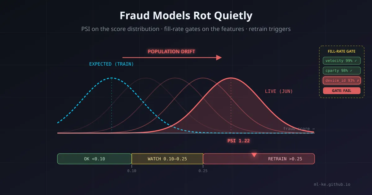
The model is a photograph of a population
A fraud model is a snapshot. It is trained on the transactions, accounts and devices of last quarter — and asked to score this quarter’s population. When those populations drift apart, the model does not crash or log an error; it quietly scores the new world with yesterday’s assumptions. In June 2025, a contractor at NCBA Bank Rwanda rewired the MTN mobile-money integration so withdrawals “succeeded” against accounts that did not exist; 70 ghost accounts moved USD 446,000 (Ksh 57.5 million) in 260 transactions over eight days before end-of-week reconciliation caught it. In April 2024, attackers moved ₦11 billion (~$7 million) out of Flutterwave to accounts across five institutions in four days — undetected because the deposits were kept below the fraud-check trigger limits.
The August 31 post asked how to detect the anomalous line; the August 20 post asked which features catch the novel attack. This post asks a different question, one layer up: how do you know the model itself has gone stale? The answer is production population monitoring — PSI on score bands, feature-drift checks, and data-quality gates on the input pipeline. It is the control that would have made both incidents visible before the money left.
Why fraud models rot silently
Fraud is adversarial drift. Unlike churn or credit models, where population change is mostly passive (the economy moved, customers aged), a fraud model faces an opponent who reads the rules and adapts. The Flutterwave pattern is the canonical case: once fraudsters know a bank flags transfers above a threshold, they split the flow into sub-threshold pieces — each line individually ordinary, the aggregate extraordinary. That is not a per-transaction anomaly; it is an engineered shift in the distribution the model sees.
Concept drift is the second rot vector. NCBA’s ghost accounts were a new pattern: synthetic accounts activating with perfect success behavior. A model trained on historical fraud sees “new account + immediate high-value activity” as risky — but if the training population never contained an insider who could fake the success side of the ledger, the model has no label for it. The feature relationships it learned are simply wrong for the new reality.
Both failure modes share a signature: the score distribution moves before the loss ledger does. The fraudster’s adaptation phase — testing thresholds, warming accounts, calibrating amounts — shifts the population weeks before the big transfer. That window is where model monitoring earns its keep.
PSI: the scorecard industry’s drift meter
The Population Stability Index (PSI) is the standard tool for watching a score distribution. It comes from credit scorecard practice — where it has monitored application populations for decades — and transfers directly to fraud scores:
\[\text{PSI} = \sum_{i=1}^{k} (A_i - E_i) \times \ln\left(\frac{A_i}{E_i}\right)\]where the score range is cut into $k$ bins (typically 10), $E_i$ is the share of the expected (training/reference) population in bin $i$, and $A_i$ is the share of the actual (live) population in the same bin. Bins are fixed at model build time so the comparison is apples-to-apples. The industry rule of thumb:
| PSI | Interpretation | Action |
|---|---|---|
| < 0.10 | Little change | No action |
| 0.10 – 0.25 | Moderate shift | Investigate drivers, watch next period |
| > 0.25 | Significant shift | Treat as retrain trigger, backtest challenger |
PSI is deliberately crude — no p-values, no normality assumptions — which is exactly why it works as a production tripwire: cheap to compute hourly or daily, robust to large data, and interpretable by the fraud team that owns the alert.
A month-by-month simulation
Here is the failure mode made concrete. A mobile-money fraud model trained in January scores every withdrawal 0–100 (higher = riskier). From April, fraudsters begin splitting transfers into amounts just under the alert threshold. Every single transaction still scores “normal” per-line — no rule fires, no anomaly detector trips. But the population of scores creeps right, month over month:
1
2
3
4
5
6
7
8
9
10
11
12
13
14
15
16
17
18
19
20
21
22
23
24
25
26
27
28
29
30
31
32
33
34
35
36
37
38
39
40
41
42
43
import math, random
from collections import Counter

random.seed(42)

def score_population(n, shift=0.0):
    out = []
    for _ in range(n):
        s = random.gauss(38.0 + shift * 14.0, 9.0)   # baseline mean ~38
        s = max(0.0, min(100.0, s))
        if random.random() < 0.18 * shift:           # sub-threshold bump
            s = random.uniform(55.0, 70.0)           # stays below the alert
        out.append(s)
    return out

def psi(expected, actual, bins=10, lo=0.0, hi=100.0):
    width = (hi - lo) / bins
    edges = [lo + i * width for i in range(bins + 1)]
    exp_c = Counter(); act_c = Counter()
    for v in expected:
        exp_c[min(int((v - lo) / width), bins - 1)] += 1
    for v in actual:
        act_c[min(int((v - lo) / width), bins - 1)] += 1
    n_e, n_a = len(expected), len(actual)
    total = 0.0; rows = []
    for b in range(bins):
        e = max(exp_c[b] / n_e, 1e-4)   # guard against empty bins
        a = max(act_c[b] / n_a, 1e-4)
        contrib = (a - e) * math.log(a / e)
        rows.append((f"[{edges[b]:.0f}-{edges[b+1]:.0f})", e, a, contrib))
        total += contrib
    return total, rows

train = score_population(40000, shift=0.0)
periods = [("Jan", 0.00), ("Feb", 0.00), ("Mar", 0.05),
           ("Apr", 0.18), ("May", 0.32), ("Jun", 0.65)]
print(f"{'period':<10} {'PSI vs train':>12}   zone")
for name, sh in periods:
    pop = score_population(40000, shift=sh)
    v, _ = psi(train, pop)
    zone = ("OK (<0.10)" if v < 0.10 else
            "WATCH (0.10-0.25)" if v < 0.25 else "RETRAIN (>0.25)")
    print(f"{name:<10} {v:>10.3f}   {zone}")
Running it produces:
1
2
3
4
5
6
7
period     PSI vs train   zone
Jan             0.000   OK (<0.10)
Feb             0.000   OK (<0.10)
Mar             0.012   OK (<0.10)
Apr             0.121   WATCH (0.10-0.25)
May             0.344   RETRAIN (>0.25)
Jun             1.223   RETRAIN (>0.25)
The model’s detection never fired — there was no single suspicious transaction to catch. But by May the population PSI is screaming RETRAIN, a full month before the losses would have peaked. The bin table for June shows where the mass went: the 50–70 score band — the “risky but not alert-worthy” zone — grew from ~9% of the population at training to ~44% live. That is the fraudsters’ adaptation footprint, and PSI reads it like a fingerprint.
Data-quality gates: the drift you cannot see in scores
Score drift catches population change, but there is a subtler failure: feature drift hiding inside the pipeline. If a device-fingerprint vendor starts returning nulls, or an integration silently stops populating a velocity feature, the model does not see “fewer risky transactions” — it sees a feature it was trained to trust, now missing, and it falls back to weaker signals. The score distribution can look stable while the model slowly goes blind.
The fix is a fill-rate gate on every feature the model depends on, checked per batch, before scoring:
1
2
3
4
5
6
7
device_id feature fill-rate by month (gate: <95% -> investigate):
  Jan:  99.4%  PASS
  Feb:  99.2%  PASS
  Mar:  99.0%  PASS
  Apr:  98.1%  PASS
  May:  96.0%  PASS
  Jun:  93.1%  FAIL
In this (simulated) run, the feature silently degraded for five months — 99.4% → 93.1% — while the fraud score stayed inside its expected band, because the model compensated by leaning on other features. The gate is what forces the investigation: why did device_id coverage drop? (Vendor contract change? SDK update? A fraudster who learned that null-device transactions skip the device-risk score?) Fill-rate is the cheapest monitoring you can buy, and it catches the failure class PSI on scores cannot.
How we can do better
- Score PSI weekly, feature PSI monthly. Compute PSI on the fraud score against the training population every week (10 fixed bins); run the same on the top 10–20 features monthly. Alert at 0.10, escalate at 0.25.
- Publish the retrain trigger in advance. Decide what a >0.25 PSI means before it happens: freeze the challenger, backtest it on the drifted window, promote if it holds. Otherwise the alert lands in a meeting with no decision rule.
- Gate every batch on feature fill-rate. One threshold per critical feature (device_id, velocity, counterparty history), paged to the ML engineer when breached — not filed in a dashboard.
- Watch the operational canaries too. Danske Bank, before its Teradata ML overhaul, was drowning in up to 1,200 false positives per day, 99.5% of investigated cases not fraud. A rising FP rate is concept drift in disguise: the model’s decision boundary no longer matches the fraud the bank actually sees.
- Log the score distribution, not just the decision. Keep the raw scores and features per period (or a sample) so PSI is computable retroactively when an incident surfaces — NCBA’s eight days and Flutterwave’s four days were reconstructed after the fact; monitoring data is what lets you replay them.
- Treat monitoring as the adversary’s clock. Fraudsters probe thresholds and warm accounts for weeks. Every day of drift visibility is a day of adaptation the fraud team can price in before the big transfer.
Key takeaways
| Control | Catches | Blind spot |
|---|---|---|
| Per-line rules / anomaly detection | Single suspicious transactions | Distributed sub-threshold attacks (Flutterwave ₦11B) |
| Score PSI (weekly) | Population shift before losses peak | Feature failures that leave scores stable |
| Feature drift PSI | Input distribution change | Missing-data degradation hidden by fallbacks |
| Fill-rate gates | Pipeline/vendor breakage, evasion via nulls | Nothing — cheapest control you own |
| FP-rate trend | Decision boundary vs. reality mismatch | — |
References
- TechCabal — Exclusive: Flutterwave loses ₦11 billion in security breach
- Techpoint Africa — Flutterwave’s ₦11 billion breach
- Business Insider Africa — Fintech giant Flutterwave loses ₦11 billion to security breach
- Fiddler AI — Measuring Data Drift with the Population Stability Index
- Coralogix — A Practical Introduction to Population Stability Index (PSI)
- Yildirim & Ildeniz — Statistical Properties of the Population Stability Index (ResearchGate)
- NCBA Bank Rwanda ghost-account incident — Kenyans Insights, 254 News, Business Daily Africa coverage (event library, editorial-calendar.md)
- Teradata — Danske Bank fraud ML case study and Fintech Futures (1,200 FPs/day; ~50% FP reduction)