Thirty Times Smaller: Auditing Embedding Compression Before You Ship It

Introduction

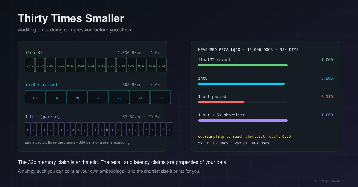
A hundred million 384-dimension embeddings occupy 153.6 GB of RAM as float32. That single number is why quantization migrated from research papers into default settings in vector databases: convert each component to 8 bits and the corpus fits in a quarter of the machine; keep only the sign of each component and it fits in a twenty-ninth. The compression ratios are honest arithmetic. What is not arithmetic is what happens next.

Three claims travel together in vendor documentation: 32x less memory, roughly the same answers, and faster search. The first is arithmetic you can check with a calculator. The other two are properties of your data and your implementation — and they decide whether the compressed index is shippable.

The framing This is about the representation itself — not the denominator of the recall number (The Denominator Is the Metric), not the serving engine (vLLM and LLM Serving, Model Serving 101), and not how an agent stores memory (Memory Systems for AI Agents). Five runnable blocks below: the memory arithmetic, a corpus you control, what the rescore reads, the speed comparison every vendor post skips, and an audit() function you can point at your own embeddings.

The short version of what follows: int8 was nearly free, 1-bit was catastrophic alone and free once paired with a shortlist, dropping dimensions was a flat loss, and the speed advantage everyone repeats did not appear in a reference implementation at all.

The one claim that is arithmetic

Start with what cannot be argued about. For a 384-dimension embedding:

"""Block 1: the memory bill, computed rather than quoted."""
D = 384
N = [1_000_000, 10_000_000, 100_000_000]
representations = [
    ("float32 (baseline)", D * 4),
    ("int8 + per-vector scale", D * 1 + 4),
    ("1-bit packed + norm", D // 8 + 4),
]

print(f"dims = {D}")
print(f"{'representation':26s} {'bytes/vec':>10s} {'ratio':>7s} {'@1M':>9s} {'@10M':>9s} {'@100M':>10s}")
base = representations[0][1]
for name, b in representations:
    sizes = " ".join(f"{b * n / 1e9:8.1f}G" for n in N)
    print(f"{name:26s} {b:10d} {base / b:6.1f}x {sizes}")

print(f"\nvectors that fit in 16 GB of RAM")
for name, b in representations:
    print(f"  {name:26s} {16e9 / b / 1e6:8.1f} M")

print(f"\npopcount words per candidate: {D // 8} bytes = {D // 64} x uint64")
print(f"bits compared per candidate: {D}")

The interesting detail is the third row: the raw sign bits are 48 bytes — exactly 32x smaller, matching the figure in the Sentence Transformers quantization write-up — but you usually also keep a 4-byte norm per vector for cosine rescoring, which brings the real number to 52 bytes and 29.5x. That is the first place a quoted compression ratio drifts from a deployed one: 32x is the codebook, 29.5x is what you store.

The capacity column is the part worth internalising: a 16 GB node that holds 10.4 million float32 vectors holds 41.2 million int8 vectors and 307.7 million 1-bit ones. For a 40-million-vector corpus, quantization is not an optimisation — it is the difference between one node and four.

Four ways to shrink a vector, and what each one breaks

Representation	Mechanism	Compression	What it actually costs
Scalar (int8)	Per-vector max-abs scale, round each component to one of 256 levels	4.0x	A bounded per-coordinate error of |max|/254; ranking noise only where neighbours are near-ties
Binary (1-bit)	Threshold each component of a normalised vector at 0	32x (29.5x with norms)	Magnitude is gone; Hamming distance only tracks angular distance well when the distribution is centred
Dimension truncation	Keep the first n components of an MRL-trained vector	4x at 96 of 384 dims	Unrecoverable information loss on any embedding not trained for it
Product / variable-bit	Split into subvectors, codebook or non-uniform bucket allocation	up to 64x	Needs training, codebooks, and its own recall audit

Qdrant’s quantization guide describes scalar quantization as “4x compression with minimal accuracy loss” and binary as “up to 32x compression”, with the caveat that binary is “best suited for high-dimensional, centered vector distributions”. That caveat is the whole difficulty. Real embedding models do not produce centred, isotropic vectors — they produce anisotropic ones where early dimensions carry far more variance than late ones. Qdrant’s newer TurboQuant mode applies “a fast random rotation to vectors before compression, which evenly redistributes data across coordinates”, explicitly to “overcome a key limitation found in binary quantization”. A rotation step shipped ahead of binarization is the tell: sign-only storage is fragile on raw embeddings.

The rank ordering itself is simple enough to state exactly. For two normalised vectors $x$ and $q$:

\[\lVert x - q \rVert^2 = 2 - 2\,x \cdot q\]

so ranking by cosine similarity and ranking by Euclidean distance are the same ordering, and any monotone transform of either is a valid retrieval score. Binary quantization replaces $x$ with $\operatorname{sign}(x)$, and Hamming distance counts the positions where the two sign patterns disagree. Hamming is monotone in angular distance only in expectation for random unit vectors; on structured data it is an approximation you have to measure.

What it costs on a corpus you control

Public retention figures are measured on public benchmarks, which is exactly the wrong corpus for a decision about your index. So measure. The block below builds a synthetic corpus with the properties that matter — cluster structure, unequal per-dimension spread, tunable separability — and an exact float32 search as ground truth.

"""What embedding compression costs: measured, not quoted.

Synthetic corpus with controllable separability (clustered + anisotropic, like real
embedding spaces). Ground truth is exact float32 search over the same vectors.
"""
import numpy as np

K = 10
D = 384


def make_corpus(n_docs, n_queries, dim=D, n_clusters=400, noise=0.3, seed=7, decay=0.2):
    rng = np.random.default_rng(seed)
    dim_scale = (np.arange(dim) + 1.0) ** -decay               # unequal dimension spread
    dim_scale /= np.linalg.norm(dim_scale)
    centers = rng.normal(size=(n_clusters, dim)) * dim_scale
    centers /= np.linalg.norm(centers, axis=1, keepdims=True)
    docs = centers[rng.integers(0, n_clusters, n_docs)] + noise * dim_scale * rng.normal(size=(n_docs, dim))
    queries = centers[rng.integers(0, n_clusters, n_queries)] + noise * dim_scale * rng.normal(size=(n_queries, dim))
    docs /= np.linalg.norm(docs, axis=1, keepdims=True)
    queries /= np.linalg.norm(queries, axis=1, keepdims=True)
    return docs.astype(np.float32), queries.astype(np.float32)


def recall(cand, truth, k=K):
    """Fraction of the exact top-k that survives a candidate list."""
    return float(np.mean([len(set(c) & set(t)) / k for c, t in zip(cand, truth)]))


def top_k(scores, k=K):
    return np.argsort(-scores, axis=1)[:, :k]


def to_int8(x):
    scale = np.abs(x).max(axis=1, keepdims=True) / 127.0
    return np.round(x / scale).astype(np.int8), scale.astype(np.float32)


def hamming(packed_q, packed_d):
    """Hamming distance between packed sign vectors: XOR, then popcount."""
    return np.stack([np.bitwise_count(packed_q[i] ^ packed_d).sum(axis=1)
                     for i in range(packed_q.shape[0])])


docs, queries = make_corpus(10_000, 200)
truth = top_k(queries @ docs.T)
print(f"corpus {docs.shape[0]:,} x {docs.shape[1]}  queries {queries.shape[0]}  k={K}")

# Is the ground truth even stable? Nudge each query by 1% and look again.
dim_scale = (np.arange(D) + 1.0) ** -0.2
dim_scale /= np.linalg.norm(dim_scale)
rs = np.random.default_rng(0)
nudged = (queries + 0.01 * dim_scale * rs.normal(size=queries.shape)).astype(np.float32)
print(f"ground-truth stability (1% query nudge): {recall(top_k(nudged @ docs.T), truth):.3f}")

d8, s8 = to_int8(docs)
db, qb = np.packbits(docs > 0, axis=1), np.packbits(queries > 0, axis=1)
ham = hamming(qb, db)

single = {
    "float32 (exact)": 1.0,
    "int8": recall(top_k((queries @ d8.T.astype(np.float32)) * s8.ravel()), truth),
    "1-bit packed": recall(np.argsort(ham, axis=1)[:, :K], truth),
}
for d in (96, 192):
    t = docs[:, :d] / np.linalg.norm(docs[:, :d], axis=1, keepdims=True)
    tq = queries[:, :d] / np.linalg.norm(queries[:, :d], axis=1, keepdims=True)
    single[f"first {d} dims only"] = recall(top_k(tq @ t.T), truth)

print("\nsingle-stage recall@10")
for name, val in single.items():
    print(f"  {name:22s} {val:.3f}")

for n_docs in (10_000, 100_000):
    if n_docs > 10_000:                                  # rebuild larger, same parameters
        docs_n, queries_n = make_corpus(n_docs, 200)
        truth_n = top_k(queries_n @ docs_n.T)
        ham_n = hamming(np.packbits(queries_n > 0, axis=1), np.packbits(docs_n > 0, axis=1))
    else:
        docs_n, queries_n, truth_n, ham_n = docs, queries, truth, ham
    print(f"\nshortlist recall + rescore ({n_docs:,} docs, 1-bit candidates, float32 rerank)")
    print(f"  {'oversampling':>13s} {'R':>7s} {'shortlist recall':>17s} {'after rescore':>14s}")
    for mult in (1, 2, 5, 25, 50):
        cand = np.argsort(ham_n, axis=1)[:, :K * mult]
        g = np.stack([c[np.argsort(-(docs_n[c] @ queries_n[i]))[:K]] for i, c in enumerate(cand)])
        print(f"  {mult:12d}x {K*mult:7d} {recall(cand, truth_n):17.3f} {recall(g, truth_n):14.3f}")

Read it in order, because the first line changes how to interpret the rest:

• Ground-truth stability 0.988. Nudging each query by 1% of its norm keeps 98.8% of the exact top-10. Had this come out near 0.6, every compression figure below would be noise about a set that is not even well defined. Check it before anything else — the same discipline as auditing a metric’s denominator, applied to the query side.
• int8: 0.965. A 3.5% loss of the exact top-10 for a 4x memory cut. This is the row that matches the marketing, and it is the default choice for good reason.
• 1-bit alone: 0.516. Half the top-10 survives sign-only search. Compare that with the widely quoted “~92.5% of retrieval performance without rescoring” from the Sentence Transformers write-up and the difference is instructive rather than contradictory: their figure is retention on a benchmark with graded relevance across a large judged set, mine is exact top-10 set overlap on 400 clusters where the top-10 are often near-ties. Same quantizer, different question. What is transferable is the shape of the answer: sign-only ranking is a candidate generator, not a ranker.
• First 96 dims only: 0.758. First 192: 0.826. Dimension truncation is a flat loss here — it does not improve as the corpus gets easier to separate, because it discards information rather than adding noise. Those numbers are what truncation looks like on vectors that were never trained for it. On an MRL-trained model it is a different story: the same write-up reports 93.1% retention at 12x compression for text-embedding-3-large, 95.8% at 3x for nomic-embed-text-v1.5. Truncation is a property of the model, not a free knob.

The shortlist is the whole trick

If 1-bit search finds half the exact top-10, the fix is not a better 1-bit quantizer — it is to retrieve more candidates cheaply and then re-rank them expensively. This is the rescore step Yamada et al. introduced, described in the Sentence Transformers write-up: “we first retrieve rescore_multiplier * top_k results with the binary query embedding and the binary document embeddings… and then rescore that list of binary document embeddings with the float32 query embedding,” which “preserve[s] up to ~96% of the total retrieval performance, while reducing the memory and disk space usage by 32x”. Vespa’s Matryoshka and binary vectors post puts post-rescore retention at “95-96% of using the original float representations”.

The multiplier is the number nobody publishes per-corpus, and it is the only one your latency budget cares about. From the same run:

Oversampling	R	Shortlist recall (10k docs)	After float32 rescore
1x	10	0.516	0.516
2x	20	0.872	0.872
5x	50	1.000	1.000
25x	250	1.000	1.000

And at 100,000 documents, same code, same corpus parameters:

Oversampling	R	Shortlist recall	After float32 rescore
2x	20	0.207	0.207
10x	100	0.667	0.667
25x	250	0.995	0.995
50x	500	1.000	1.000

Two things fall out of that pair of tables. First, the oversampling factor you need grows with corpus size — 5x reached perfect shortlist recall at 10k vectors, 25x at 100k. Second, Qdrant’s documented search example passes "rescore": true, "oversampling": 2.0. Those are reasonable defaults for the corpora they were tuned on. In my corpus, 2x delivered 0.872 shortlist recall at 10,000 vectors and 0.207 at 100,000 — and the rescore stage then ranks a candidate list that mostly does not contain the answer. That is the worst kind of failure: the pipeline looks like it is working and returns confidently wrong neighbours. Inherit the code, not the constant.

What the rescore costs is bounded and small, which is the actual argument for this design:

"""Block 4: what compression does to the bytes you actually move per query."""

D = 384
N = 100_000_000
BW_GBPS = 20.0            # single-node memory bandwidth, ~10-30 GB/s typical

float32_bytes = D * 4
bit_bytes = D // 8 + 4

print("full scan of the index, per query")
print(f"  float32:  {N * float32_bytes / 1e9:8.1f} GB  -> {N * float32_bytes / 1e9 / BW_GBPS:8.3f} s  "
      f"({1 / (N * float32_bytes / 1e9 / BW_GBPS):.3f} QPS)")
print(f"  1-bit:    {N * bit_bytes / 1e9:8.1f} GB  -> {N * bit_bytes / 1e9 / BW_GBPS:8.3f} s  "
      f"({1 / (N * bit_bytes / 1e9 / BW_GBPS):.3f} QPS)")

print("\nshortlist rescore, per query (what you read a second time)")
for mult in (2, 5, 25):
    R = 10 * mult
    rows_b = R * float32_bytes
    rows_i8 = R * (D + 4)
    print(f"  {mult:2d}x (R={R:4d}): float32 rows {rows_b / 1024:8.1f} KB   int8 rows {rows_i8 / 1024:8.1f} KB   "
          f"1-bit rows {R * bit_bytes / 1024:8.1f} KB")

print("\nif the scan happens inside an HNSW graph over the bits, not a flat scan")
for visited_pct in (0.1, 1.0, 5.0):
    visited = N * visited_pct / 100
    print(f"  {visited_pct:4.1f}% of vectors visited ({visited / 1e6:6.1f}M): "
          f"{visited * bit_bytes / 1e9:6.3f} GB per query -> {visited * bit_bytes / 1e9 / BW_GBPS * 1000:6.2f} ms")

The 25x shortlist reads 375 KB of float32 rows per query, or 95 KB if you keep int8 vectors for rescoring — a rounding error next to a page. Note the flat-scan numbers in the same output: at 100 million vectors a brute-force scan over even the packed bits moves 5.2 GB per query, which at 20 GB/s of memory bandwidth is 0.26 s. Compressing the vectors does not remove the need for an index; it changes what the index stores. Inside a graph that visits 1% of the vectors, the same scan is 2.6 ms. Vespa makes the same point from the other direction — “~1 billion hamming distance calculations per second, roughly 7x more than prenormalized angular distance… More candidates evaluated = better recall” — the speed is what buys the larger shortlist.

The speed claim is an implementation property

That brings up the last claim, and the one place my measurements flatly disagreed with the literature: Hamming distance over packed bits is supposed to be dramatically faster than float math, “2 CPU cycles” per comparison per the Sentence Transformers write-up. Measured here, in numpy, on identical vectors:

"""Is packed Hamming search actually faster? Same vectors, three ways, best of 3."""
import time
import numpy as np

N, D, Q = 10_000, 384, 200
rng = np.random.default_rng(0)
docs = rng.normal(size=(N, D)).astype(np.float32)
docs /= np.linalg.norm(docs, axis=1, keepdims=True)
queries = rng.normal(size=(Q, D)).astype(np.float32)
queries /= np.linalg.norm(queries, axis=1, keepdims=True)
db, qb = np.packbits(docs > 0, axis=1), np.packbits(queries > 0, axis=1)


def best_of(fn, reps=3):
    times = []
    for _ in range(reps):
        t0 = time.perf_counter()
        fn()
        times.append(time.perf_counter() - t0)
    return min(times)


def ham_popcount(q, d):
    return np.stack([np.bitwise_count(q[i] ^ d).sum(axis=1) for i in range(q.shape[0])])


def ham_unpack(q, d):
    return np.stack([np.unpackbits(q[i] ^ d, axis=1).sum(axis=1) for i in range(q.shape[0])])


n_dist = Q * N
print(f"numpy {np.__version__} | {N:,} vectors x {D} dims | {Q} queries | {n_dist:,} distances")
t_matmul = best_of(lambda: queries @ docs.T)
t_popcount = best_of(lambda: ham_popcount(qb, db))
t_unpack = best_of(lambda: ham_unpack(qb, db))
for name, t in (("float32 matmul (BLAS)", t_matmul),
                ("packed, bitwise_count", t_popcount),
                ("packed, unpackbits", t_unpack)):
    print(f"  {name:24s} {t*1000:7.0f} ms  {n_dist/t/1e6:7.1f} M distances/s  "
          f"{t/t_matmul:5.2f}x the matmul time")
print(f"  identical distances: {np.array_equal(ham_popcount(qb, db), ham_unpack(qb, db))}")
print(f"  packed bytes per vector: {D // 8}  popcount words: {D // 64} x uint64")

The packed search is 17x slower than the plain float32 matmul with bitwise_count, and 78x slower with the naive unpackbits path that most tutorials show — 15.1 million distances per second against 262.7 million for BLAS. Both packed paths return identical distances (the script asserts it), so the difference is purely cost, not correctness. Ratios drift run to run on a throttling laptop CPU — across six comparisons while writing this, the bitwise_count penalty ranged from 5x to 20x and the unpackbits penalty from 37x to 78x — but the ordering never flipped: numpy’s packed search was slower than the BLAS matmul it is supposed to beat, every single time. Two lessons:

1. np.bitwise_count is the popcount you want — added in NumPy 2.0 and 4x to 8x faster across runs than unpacking each byte to 8 floats, with identical distances. On older numpy, use np.unpackbits and accept the cost, or move the search out of numpy.
2. The 7x-over-angular-distance figure comes from an engine where popcount is a single hardware instruction over packed 64-bit words, in the same process that owns the index. Numpy’s byte-wise XOR-and-popcount on a separate array gets none of that: BLAS matmul is SIMD- and cache-optimised, and numpy is not, so the comparison inverts on this machine.

The honest rule that follows: the memory claim is arithmetic you can check with a calculator; the latency claim is a property of your engine and your hardware. If a design review promises a latency win from binarization, the reviewer should be shown a benchmark, not a blog post.

How to apply this

Everything above reduces to one decision procedure. Point this at your own vectors and read the last line:

"""Block 3: audit any embedding matrix before you compress it.

Replace `embeddings` with your own (N, D) float32 matrix -- e.g.
np.load("embeddings.npy") straight out of your vector store's dump.
"""
import numpy as np


def audit(embeddings, k=10, n_queries=200, candidates=(2, 5, 10, 25, 50), seed=0, target=0.99):
    x = np.asarray(embeddings, dtype=np.float32)
    x = x / np.linalg.norm(x, axis=1, keepdims=True)

    rng = np.random.default_rng(seed)
    held = rng.choice(x.shape[0], size=min(n_queries, x.shape[0] // 4), replace=False)
    mask = np.ones(x.shape[0], dtype=bool)
    mask[held] = False
    docs, queries = x[mask], x[held]                      # hold queries out of the index

    truth = np.argsort(-(queries @ docs.T), axis=1)[:, :k]
    db, qb = np.packbits(docs > 0, axis=1), np.packbits(queries > 0, axis=1)
    ham = np.stack([np.bitwise_count(qb[i] ^ db).sum(axis=1) for i in range(qb.shape[0])])

    def overlap(cand):
        return float(np.mean([len(set(c) & set(t)) / k for c, t in zip(cand, truth)]))

    report = {
        "vectors": int(x.shape[0]),
        "dims": int(x.shape[1]),
        "bytes/vector float32": int(x.shape[1] * 4),
        "bytes/vector 1-bit": int(x.shape[1] // 8 + 4),
        "1-bit recall@k alone": round(overlap(np.argsort(ham, axis=1)[:, :k]), 3),
        "min oversampling for target": None,
    }
    for mult in candidates:
        cand = np.argsort(ham, axis=1)[:, :k * mult]
        hop = round(overlap(cand), 3)
        report[f"shortlist {k * mult}"] = hop
        if report["min oversampling for target"] is None and hop >= target:
            report["min oversampling for target"] = mult
    if report["min oversampling for target"] is None:
        report["verdict"] = "1-bit candidates never reach the target here - use int8 or keep float32"
    elif report["min oversampling for target"] <= 5:
        report["verdict"] = "1-bit shortlist + float32 rescore is safe; index the bits"
    else:
        report["verdict"] = f"1-bit works, but budget {report['min oversampling for target']}x candidates"
    return report


if __name__ == "__main__":
    # Demo matrix: swap in np.load("embeddings.npy") to audit the real thing.
    rng = np.random.default_rng(7)
    dim_scale = (np.arange(384) + 1.0) ** -0.2
    dim_scale /= np.linalg.norm(dim_scale)
    centers = rng.normal(size=(400, 384)) * dim_scale
    centers /= np.linalg.norm(centers, axis=1, keepdims=True)
    emb = centers[rng.integers(0, 400, 8_000)] + 0.3 * dim_scale * rng.normal(size=(8_000, 384))

    for key, value in audit(emb).items():
        print(f"{key:32s} {value}")

The verdict line and the min oversampling for target key are what go in the design doc: the first says whether a bit index is viable at all, the second is the search parameter to configure instead of the vendor default. Then apply the table:

Your constraint	Representation	What to verify before shipping
RAM-bound, quality-first	int8 (4x)	Recall drop under 1% on your own queries; a bounded per-coordinate error
RAM-bound, latency-critical	1-bit index + shortlist + full-precision rescore	Shortlist recall at your chosen multiplier is 0.99+, not 0.9
Corpus of millions, self-hosted	1-bit index, int8 or float32 rows paged for rescoring	Bytes read per query, and that the rescore fits the latency budget
Model trained with MRL (mxbai, nomic-embed, text-embedding-3, EmbeddingGemma)	Truncate dimensions, then binarize the prefix	Per-prefix recall — the two savings multiply, but so do the losses
Arbitrary embedding, you want fewer dims	Neither — keep the dims	Truncation is not a knob on a model that was not trained for it
Under a million vectors, RAM is not binding	Nothing	Compression buys you nothing you currently need

Two operational notes that outlive the benchmark. Store the quantizer with the vectors: the per-vector scale for int8, the norm for cosine rescoring on packed bits, the sign convention — a compressed index is a format, and a format needs a version. Re-run the audit when the model or corpus changes, because retention is a property of a particular embedding distribution. The newest work in this area makes the same point structurally: Quantization Beyond Uniform Bit Allocation (VecDB workshop, VLDB 2026) finds non-uniform bit allocation beating uniform allocation at identical storage budgets, “up to 8% for PQ and up to 18% for SQ”, with the largest gains “in the low-bit regime, where uniform allocation is particularly inefficient for MRL embeddings”. Uniform, structure-blind compression leaves accuracy on the table, and how much depends on your embeddings.

On constrained hardware this stops being an optimisation exercise at all. Where RAM or a metered uplink is the binding constraint — self-hosted inference (Self-Hosting Open-Weight LLMs), edge and on-device retrieval (Edge AI in African Markets), deliberately small serving footprints (MLOps in Constrained Environments) — the representation is chosen for you, and the audit is how you find out what you just gave up.

Key takeaways

Finding	Number from this run	What to do with it
Compression ratios are arithmetic	1536 B -> 388 B -> 52 B per 384-dim vector	Check the ratio including scales and norms
int8 is close to free	recall@10 0.965 vs 1.000 exact	Default choice; verify on your own queries
Sign-only ranking is not a ranker	0.516 recall@10 alone	Always pair it with a full-precision rescore
The shortlist is what saves 1-bit	1.000 at 5x (10k docs), 25x needed at 100k	Measure the multiplier per corpus; do not inherit 2.0
Dimension truncation is a model property	0.758 at 96 dims on non-MRL vectors	Only truncate MRL-trained embeddings
The speed claim is an implementation property	packed numpy 15.1M distances/s vs 262.7M BLAS	Benchmark the engine, not the format
Use the right popcount	np.bitwise_count (NumPy 2.0+) 4.5x faster than unpackbits, identical distances	One-line fix in any numpy reference implementation
Bytes moved, not bytes stored, set the latency	5.2 GB scanned per query at 100M vectors	Keep an index over the bits; page full-precision rows

References

1. Sentence Transformers / Hugging Face, Binary and Scalar Embedding Quantization — threshold at 0, 32x reduction, Hamming at “2 CPU cycles”, the Yamada et al. rescore recipe, ~92.5% retention without rescoring and ~96% with, MRL figures.
2. Qdrant, Quantization guide — scalar (4x), binary (up to 32x, “centered vector distributions”), product (up to 64x), TurboQuant bit depths, and the rescore / oversampling: 2.0 parameters.
3. Vespa, Embedding Tradeoffs, Quantified — “~1 billion hamming distance calculations per second, roughly 7x more than prenormalized angular distance”, 32x storage, rescoring modes.
4. Vespa, Matryoshka and Binary vectors: Slash vector search costs — post-rescore retention “95-96% of using the original float representations”.
5. Sreeramji et al., Quantization Beyond Uniform Bit Allocation, VecDB workshop at VLDB 2026 — up to +8% recall (PQ) and +18% (SQ) at identical storage.
6. NumPy, numpy.bitwise_count — popcount ufunc added in NumPy 2.0.
7. Sentence Transformers, Embedding Quantization example — quantize_embeddings(..., precision="binary") and binary/ubinary packing.

Related posts

• The Denominator Is the Metric: Auditing a RAG Retriever Before You Blame the Model
• Model Serving 101: From Jupyter notebook to production API endpoint
• Edge AI in African Markets: On-device ML and offline-capable models
• MLOps in Constrained Environments