Your WHERE Clause Ate the Recall: Sizing the Candidate Pool Behind Filtered Vector Search

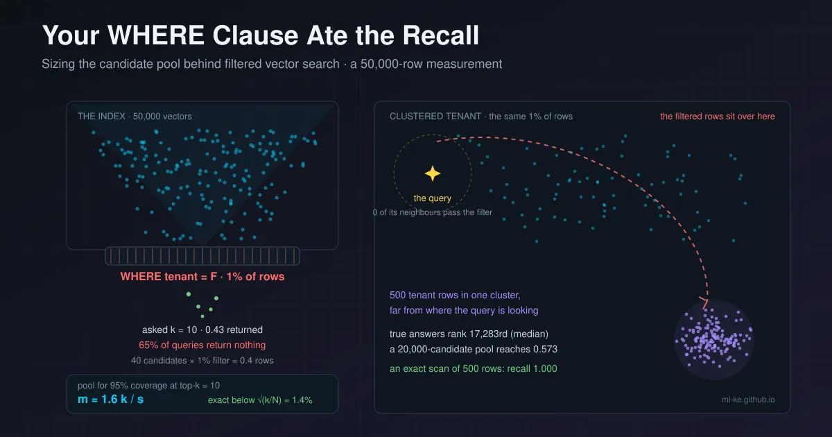
A vector index returns candidates. The filter decides how many of them answer. pgvector’s documentation gives the arithmetic: with the default hnsw.ef_search = 40 and a condition matching 10% of rows, about four rows survive the filter. This post measures that collapse, derives the pool size that fixes it, and finds the selectivity at which scanning the matching rows exactly is simply the cheaper plan.

Ask a retriever for ten documents from one tenant and it hands back four. Nothing errors: the embedding model is fine, the index built cleanly, the query vector is correct. What happened is that the nearest neighbours were computed over the whole corpus and the tenant filter was applied to whatever came back.

That ordering is not a bug in any one library. An HNSW or IVF index navigates toward the query using distance alone, so it has no way to skip rows that will fail a predicate later. PostgreSQL’s pgvector states the consequence in its own README, next to the setting that controls it: “With approximate indexes, filtering is applied after the index is scanned. If a condition matches 10% of rows, with HNSW and the default hnsw.ef_search of 40, only 4 rows will match on average.” The AWS Database Blog repeats the same figure in its write-up of pgvector 0.8.0, calling the failure overfiltering and noting that affected queries “might return fewer results than expected, or even none at all.”

This is a different question from the two retrieval posts already on the blog. The denominator is the metric was about measuring recall honestly, and the embedding compression audit about what bit packing costs. This one covers the interface between the index and the predicate sitting on top of it, and it has a computable answer: given the selectivity of your filter and your k, some pool size restores recall, and below some selectivity you should stop using the approximate index at all.

The pool is the budget, and the filter spends it

Think of the query as two stages that do not talk to each other. Stage one is the index: it returns the $m$ nearest candidates by distance, where $m$ is ef_search, nprobe or whatever your engine calls the candidate budget. Stage two is the predicate: it keeps the candidates that satisfy it. With selectivity $s$, the number of survivors is a hypergeometric draw with mean $m \cdot s$.

That single expression explains the symptom list. Ask for $k = 10$ with ef_search = 40 and a 1% filter and the expected number of survivors is 0.4, so most queries return nothing at all. Raise selectivity to 50% and the same pool yields 20 survivors, comfortably enough. Nothing about the vectors changed between those two queries. Only the arithmetic did.

There is a second, less obvious consequence of the ordering, and it is good news. If stage one returns the true top $m$ by distance and stage two sorts the survivors and keeps $k$, every row you return is genuinely in the filtered top $k$: a returned row $x$ is inside the global top $m$ and passes the filter, so any filtered row $y$ closer than $x$ would also be in the pool and would have displaced $x$ among the survivors. So recall@k collapses purely through under-return. You get too few rows, but the rows that do come back are right. The fix is sizing, not scoring, and it matters operationally because a service returning 4 of 10 looks exactly like one returning 10 of 10 with worse answers unless you count.

Measuring the collapse on one corpus

The demo below builds 50,000 unit vectors in 64 dimensions and gives them a skewed tenant column, from one large tenant at 50% of the corpus down to a small one at 1%. Metadata is assigned by row index and the vectors are independent draws, so the label carries no information about the embedding space. That independence is the assumption the arithmetic relies on, and the next section breaks it on purpose.

import numpy as np

# ---- a toy corpus whose metadata is INDEPENDENT of the embedding space ----
N, D, K = 50_000, 64, 10
NQ = 300
rng = np.random.default_rng(20261014)

X = rng.standard_normal((N, D)).astype(np.float32)
X /= np.linalg.norm(X, axis=1, keepdims=True)

# skewed tenant sizes: F is the small tenant at 1% of the corpus
sizes = {"A": 25_000, "B": 12_500, "C": 7_500, "D": 3_500, "E": 1_000, "F": 500}
lab = np.empty(N, dtype="<U1")
pos = 0
for name, n in sizes.items():
    lab[pos:pos + n] = name
    pos += n
MASK = np.stack([lab == name for name in sizes])             # (6, N) boolean

Q = rng.standard_normal((NQ, D)).astype(np.float32)
Q /= np.linalg.norm(Q, axis=1, keepdims=True)

POOL = (40, 100, 400, 1000)
hit = {(name, m): 0 for name in sizes for m in POOL}
got_n = {(name, m): 0 for name in sizes for m in POOL}
empty = {(name, m): 0 for name in sizes for m in POOL}

for i in range(NQ):
    scores = X @ Q[i]
    truth = {}
    for j, name in enumerate(sizes):
        idx = np.flatnonzero(MASK[j])
        truth[name] = set(idx[np.argpartition(-scores[idx], K)[:K]].tolist())
    for m in POOL:
        cand = np.argpartition(-scores, m)[:m]        # the ANN returns m candidates
        cand = cand[np.argsort(-scores[cand])]        # ... nearest first
        for j, name in enumerate(sizes):
            got = cand[MASK[j][cand]][:K]             # then the filter is applied
            hit[(name, m)] += len(truth[name].intersection(got.tolist()))
            got_n[(name, m)] += len(got)
            empty[(name, m)] += (len(got) == 0)

print(f"corpus {N} vectors, dim {D}, {NQ} queries, k={K}; m = candidates the index returns")
print("filter  sel.   rows   " + "".join(f"  R@10 m={m:<4}" for m in POOL) + "  got m=40  got m=1000  empty m=40")
print("-" * 84)
for name in sizes:
    s = sizes[name] / N
    row = f"{name:<7} {s:>5.1%} {sizes[name]:>6}   "
    row += "".join(f"{hit[(name, m)] / (NQ * K):>13.3f}" for m in POOL)
    row += f"{got_n[(name, 40)] / NQ:>10.2f}{got_n[(name, 1000)] / NQ:>12.2f}{empty[(name, 40)] / NQ:>12.2f}"
    print(row)
print("\nrows you expect to survive the filter in a pool of m candidates = m x selectivity")
for name in ("A", "F"):
    s = sizes[name] / N
    print(f"  tenant {name} (sel {s:.2f}): " + "  ".join(f"m={m} -> {m * s:.1f}" for m in POOL))

tenant	selectivity	rows	R@10 m=40	R@10 m=100	R@10 m=400	R@10 m=1000	returned m=40	returned m=1000	empty m=40
A	50.0%	25,000	1.000	1.000	1.000	1.000	10.00	10.00	0.00
B	25.0%	12,500	0.892	1.000	1.000	1.000	8.92	10.00	0.00
C	15.0%	7,500	0.610	0.993	1.000	1.000	6.10	10.00	0.00
D	7.0%	3,500	0.292	0.692	0.999	1.000	2.92	10.00	0.06
E	2.0%	1,000	0.078	0.196	0.742	1.000	0.78	10.00	0.46
F	1.0%	500	0.043	0.105	0.403	0.872	0.43	8.72	0.65

Read the recall column against the last one. Tenant E returns 0.78 rows on average at m = 40, so 46% of queries come back empty and recall@10 sits at 0.078. Tenant A, five times bigger, is already at 1.000 with the same pool. The expected-survivor line at the bottom of the output is the explanation: 40 candidates times 1% is 0.4, and 40 times 50% is 20.

The corpus reproduces the vendor figure as well: a 10% filter over a 40-candidate pool means 4 surviving rows, which tenants C and D bracket at 6.10 and 2.92. And the under-return is what gets filed as a bug report. At m = 40, 65% of queries against a 1% filter return zero rows, and a RAG pipeline handed an empty context does not usually crash. It answers from the model’s memory or a stale cache, and the retrieval miss surfaces as a hallucination two layers away from where it happened.

Sizing the pool from two numbers you already have

If the pool is the budget, the fix is to spend it deliberately: how much candidate budget buys confidence that $k$ matching rows are in hand? That is the hypergeometric tail $P(X \ge k)$, where $X$ counts matches in a pool of $m$ drawn without replacement from $N$ rows with $sN$ matching, and it inverts numerically: find the smallest $m$ whose probability clears 0.95.

import numpy as np
from math import lgamma, exp, sqrt

N, D, K = 50_000, 64, 10
NQ = 300
rng = np.random.default_rng(20261014)

X = rng.standard_normal((N, D)).astype(np.float32)
X /= np.linalg.norm(X, axis=1, keepdims=True)
Q = rng.standard_normal((NQ, D)).astype(np.float32)
Q /= np.linalg.norm(Q, axis=1, keepdims=True)

# disjoint row bands, one per selectivity: exactly s*N rows each
SEL = [0.005, 0.01, 0.02, 0.05, 0.10, 0.20, 0.50]
bands, off = {}, 0
for s in SEL:
    n = int(round(s * N))
    bands[s] = np.arange(off, off + n)
    off += n

def log_comb(n, k):
    if k < 0 or k > n:
        return float("-inf")
    return lgamma(n + 1) - lgamma(k + 1) - lgamma(n - k + 1)

def p_pool(n_rows, n_match, m, k):
    """P(at least k of the m candidates the index returns pass the filter)."""
    if m < k:
        return 0.0
    s = n_match / n_rows
    mu = m * s
    sd = sqrt(m * s * (1 - s) * (n_rows - m) / (n_rows - 1))
    top = min(m, n_match, int(mu + 8 * sd) + 5)
    logden = log_comb(n_rows, m)
    total = 0.0
    for i in range(k, top + 1):
        if m - i <= n_rows - n_match:
            total += exp(log_comb(n_match, i) + log_comb(n_rows - n_match, m - i) - logden)
    return total

def min_pool(n_rows, n_match, k, target=0.95):
    """Smallest pool that reaches `target` coverage; P grows with m, so bisect instead of scans."""
    lo, hi = k, n_rows
    while lo < hi:
        mid = (lo + hi) // 2
        if p_pool(n_rows, n_match, mid, k) >= target:
            hi = mid
        else:
            lo = mid + 1
    return lo

plan = {s: min_pool(N, len(bands[s]), K) for s in SEL}

print(f"N={N}, k={K}: cheapest candidate pool that puts k matching rows in front of the filter")
print("sel.    rows    k/s (mean pool)   m for 95% coverage   pre-filter scans   winner")
print("-" * 88)
for s in SEL:
    n_sel = len(bands[s])
    print(f"{s:>5.1%}{n_sel:>8}{int(round(K / s)):>18}{plan[s]:>21}{n_sel:>19}   "
          f"{'pre-filter' if n_sel < plan[s] else 'over-fetch'}")

hit = {s: 0 for s in SEL}
for i in range(NQ):
    scores = X @ Q[i]
    for s in SEL:
        idx = bands[s]
        truth = set(idx[np.argpartition(-scores[idx], K)[:K]].tolist())
        cand = np.argpartition(-scores, plan[s])[:plan[s]]
        cand = cand[np.argsort(-scores[cand])]
        hit[s] += len(truth.intersection(cand[np.isin(cand, idx)][:K].tolist()))

print("\nmeasured recall@10 when the pool is sized by that rule, and the multiplier it implies")
for s in SEL:
    print(f"  sel {s:>5.1%}: m={plan[s]:<6} recall@10={hit[s] / (NQ * K):.3f}   x{plan[s] / (K / s):.2f} of k/s")

print("\nthe multiplier is not a constant (95% pools at 1% selectivity, N=50,000)")
for k in (1, 5, 10, 50, 100):
    m = min_pool(N, 500, k)
    print(f"  k={k:<4} m95={m:<6} x{m / (k / 0.01):.2f} of k/s")

print(f"\nwhere the two plans cost the same number of rows: s* = sqrt(k/N) = {(K / N) ** 0.5:.4%}"
      f" with the mean pool, sqrt(1.6k/N) = {((1.6 * K) / N) ** 0.5:.4%} with the 95% pool")

selectivity	matching rows	mean pool $k/s$	pool for 95% coverage	rows a pre-filter scans	winner
0.5%	250	2,000	3,096	250	pre-filter
1.0%	500	1,000	1,557	500	pre-filter
2.0%	1,000	500	780	1,000	over-fetch
5.0%	2,500	200	311	2,500	over-fetch
10.0%	5,000	100	154	5,000	over-fetch
20.0%	10,000	50	76	10,000	over-fetch
50.0%	25,000	20	28	25,000	over-fetch

Two things fall out of it. First, the rule works: sized by it, measured recall@10 lands between 0.990 and 0.995 at every selectivity against a 0.95 target. Second, the multiplier over the mean pool $k/s$ is stable but not 1.0, sitting at 1.55 for $k = 10$ and falling as $k$ grows:

$k$	pool for 95% coverage	multiplier over $k/s$
1	298	2.98
5	909	1.82
10	1,557	1.56
50	6,128	1.23
100	11,473	1.15

A larger $k$ is a bigger absolute requirement, so the same shortfall in the tail costs proportionally less. “Fetch $k/s$ candidates” therefore under-delivers badly for small $k$, and the working rule for a top-ten retrieval call is closer to $1.6\,k/s$.

The selectivity where over-fetching stops being worth it

Now cost both plans in the same currency. The ACORN paper’s complexity analysis uses distance computations, which dominate, and gives pre-filtering $O(

X_p

) = O(sN + k)$ with perfect recall, against $O(\log n + k/s)$ for post-filtering when the filtered rows are spread uniformly. Setting the two equal in the cost that scales:

\[\frac{k}{s} = sN \quad \Longrightarrow \quad s^{*} = \sqrt{\frac{k}{N}}\]

For 50,000 rows and $k = 10$ that is 1.41%, and the measured crossover falls where it should: pre-filtering wins at 1.0% and loses at 2.0%. Substituting the 95% pool for the mean pool moves the threshold right to $\sqrt{1.6k/N} = 1.79\%$; the demo prints both, and the truth lies between them.

The crossover inverts the usual intuition. Pre-filtering is supposed to be the naive plan that “does not scale”, and on a large corpus at high selectivity it is the wrong plan. At low selectivity it scans a small set, exactly, and cannot under-return. The FANNS benchmark reaches the same conclusion, recommending filter-then-search for very low selectivity “where throughput and recall often diverge most across methods”. The 2026 system study of filtered ANN in vector databases goes further: pgvector’s optimizer “frequently selects suboptimal execution plans, favoring approximate index scans even when exact sequential scans would yield perfect recall at comparable latency”, and partition-based IVFFlat indexes “often outperform graph-based indexes (HNSW) in low-selectivity regimes”.

The case the arithmetic cannot save

Everything above assumed the filter is independent of the embedding space. Real metadata often is not: a tenant whose documents are all about one product, a label tied to one geography, a category that is semantically coherent. Those rows cluster in the vector space, and then the query’s neighbourhood and the filter’s rows sit in different places. The third block pushes the same 500-row tenant within about ten degrees of one topic direction and leaves the rest of the corpus untouched.

import numpy as np

N, D, K = 50_000, 64, 10
NQ = 300
rng = np.random.default_rng(20261014)

X = rng.standard_normal((N, D)).astype(np.float32)
X /= np.linalg.norm(X, axis=1, keepdims=True)
Q = rng.standard_normal((NQ, D)).astype(np.float32)
Q /= np.linalg.norm(Q, axis=1, keepdims=True)

POOL = (40, 400, 4000, 20_000)
rare = np.arange(500)                                 # a 1%-selectivity tenant
flag = np.zeros(N, dtype=bool)
flag[rare] = True

def unit(a):
    return a / np.linalg.norm(a, axis=-1, keepdims=True)

topic = unit(rng.standard_normal(D).astype(np.float32))     # the tenant's own topic direction

def measure(Xc):
    """Post-filter recall@10 for the 1% filter, plus two diagnostics."""
    rec = {m: 0 for m in POOL}
    ranks, local = [], []
    for i in range(NQ):
        scores = Xc @ Q[i]
        order = np.argsort(-scores)                    # full ranking, brute force
        rank_of = np.empty(N, dtype=np.int32)
        rank_of[order] = np.arange(N)
        truth = rare[np.argsort(-scores[rare])[:K]]
        ranks.extend(rank_of[truth].tolist())
        local.append(flag[order[:100]].mean() / 0.01)  # local prevalence / global selectivity
        for m in POOL:
            cand = order[:m]
            got = cand[flag[cand]][:K]
            rec[m] += len(set(truth.tolist()) & set(got.tolist()))
    return {m: rec[m] / (NQ * K) for m in POOL}, int(np.median(ranks)), float(np.mean(local))

Xun = X.copy()                                    # metadata independent of the embedding space
un, un_rank, un_gls = measure(Xun)

Xcl = X.copy()                                    # the same 500 rows, all inside ~10 degrees of one topic
Xcl[rare] = unit(topic + 0.18 * unit(rng.standard_normal((500, D)).astype(np.float32)))
cl, cl_rank, cl_gls = measure(Xcl)

print("a 1%-selectivity tenant (500 of 50,000 rows), 300 queries, k=10")
print("case              R@10 m=40  R@10 m=400  R@10 m=4000  R@10 m=20000  median rank of the 10 true answers"
      "  local prevalence / selectivity")
print("-" * 128)
print(f"{'uncorrelated':<18}{un[40]:>9.3f}{un[400]:>12.3f}{un[4000]:>13.3f}{un[20_000]:>13.3f}"
      f"{un_rank:>37}{un_gls:>32.2f}")
print(f"{'clustered':<18}{cl[40]:>9.3f}{cl[400]:>12.3f}{cl[4000]:>13.3f}{cl[20_000]:>13.3f}"
      f"{cl_rank:>37}{cl_gls:>32.2f}")
print(f"\ncluster tightness: mean cosine of the 500 clustered rows with the topic direction = "
      f"{float((Xcl[rare] @ topic).mean()):.2f}")
print(f"pre-filter (score the 500 matching rows) returns the exact top-10 in both cases: recall 1.000")
print(f"the clustered tenant needs a pool of about {cl_rank:,} rows ({cl_rank / N:.0%} of the index) before"
      f" its rows are even in view - {cl_rank / 500:.0f}x the rows a pre-filter would score")

tenant shape	R@10 m=40	R@10 m=400	R@10 m=4000	R@10 m=20000	median rank of the true answers	local prevalence / selectivity
uncorrelated	0.040	0.395	1.000	1.000	503	0.94
clustered	0.003	0.025	0.148	0.573	17,283	0.22

Same tenant size, same queries, same k. The uncorrelated tenant is fully recovered by m = 4000, the sizing rule doing its job. The clustered tenant sits at 0.148 there and reaches only 0.573 with a pool of 20,000 candidates, 40% of the whole index. The next column says why: the ten true answers rank 17,283rd on median in the global distance ordering, so no pool much smaller than that can see them. Pumping ef_search into the tens of thousands spends the latency and still misses half the queries.

The last column is the diagnostic worth keeping. Local prevalence divided by global selectivity asks “are the filtered rows where the query is looking?” and returns 0.94 when the metadata is independent, 0.22 when the tenant clusters. The 2026 system study formalizes this as Global-Local Selectivity and uses it to explain exactly this failure. Read my number honestly, though: 0.22 is not zero. Some queries do point at the cluster, which is why the clustered row still climbs to 0.573 at the deepest pool instead of sitting at zero.

A selective filter and a correlated filter are different problems. Independent metadata needs a bigger candidate pool. Correlated metadata needs a plan that starts from the filtered rows, because the answer is nowhere near the query’s neighbourhood.

What the engines actually do about it

Every serious engine has a knob or a strategy here, and they map onto the three plans the measurements distinguish.

Engine or method	Mechanism	What it costs
pgvector hnsw.iterative_scan (strict_order / relaxed_order)	keeps scanning until enough filtered rows are found; strict returns exact distance order, relaxed gives better recall	scans a larger slice of the index, bounded by hnsw.max_scan_tuples
pgvector partial index	a separate index over one filter value	the filter value must be known at build time
Milvus iterative filtering	the vector search runs in iterations, each returned entity is filtered until topK is reached	trades latency for recall stability
ACORN, Filtered-DiskANN	the predicate is built into the graph so a filtered subgraph is still navigable	index build and memory; ACORN falls back to pre-filtering below a minimum selectivity
IVFFlat / partition indexes	prune to a cluster, then filter	2026 measurements find them competitive with or better than HNSW at low selectivity

pgvector hands you the expansion knob and expects you to size it, Milvus hides the expansion behind an iteration loop, and the research indexes pay in build time to make the graph filter-aware. ACORN states the fallback rule explicitly: it is configured with a minimum selectivity $s_{min}$, below which it pre-filters instead of searching the filtered subgraph.

How to apply this

The fourth block turns the arithmetic into a decision. Feed it the corpus size, your k and the selectivity of the filter, and it returns the plan to ask for.

from math import lgamma, exp

def log_comb(n, k):
    if k < 0 or k > n:
        return float("-inf")
    return lgamma(n + 1) - lgamma(k + 1) - lgamma(n - k + 1)

def pool_for(n_rows, n_match, k, target=0.95):
    """Smallest candidate pool whose chance of holding k matching rows reaches `target`."""
    for m in range(k, n_rows + 1):
        logden = log_comb(n_rows, m)
        p = 0.0
        for i in range(k, min(m, n_match) + 1):
            if m - i <= n_rows - n_match:
                p += exp(log_comb(n_match, i) + log_comb(n_rows - n_match, m - i) - logden)
        if p >= target:
            return m
    return n_rows

def choose_plan(n_rows, k, selectivity, overfetch=1.6):
    """Which plan to ask your vector engine for, from three numbers you already have."""
    matches = int(round(n_rows * selectivity))
    crossover = (overfetch * k / n_rows) ** 0.5
    if selectivity <= crossover:
        return (f"pre-filter: score all {matches:,} matching rows, recall 1.000 "
                f"(crossover at {crossover:.2%})")
    pool = pool_for(n_rows, matches, k)
    return (f"post-filter: ask for a pool of {pool:,} candidates = {pool / n_rows:.2%} of the index "
            f"(crossover at {crossover:.2%})")

for n_rows, k, s in [(50_000, 10, 0.005), (50_000, 10, 0.02), (50_000, 10, 0.20),
                     (5_000_000, 10, 0.01), (5_000_000, 100, 0.05)]:
    print(f"rows={n_rows:>9,}  k={k:<4} selectivity={s:>6.2%}  ->  {choose_plan(n_rows, k, s)}")

Its output on five combinations, including two at five million rows:

rows	$k$	selectivity	plan
50,000	10	0.50%	pre-filter: score all 250 matching rows
50,000	10	2.00%	post-filter: pool of 780 candidates, 1.56% of the index
50,000	10	20.00%	post-filter: pool of 76 candidates, 0.15% of the index
5,000,000	10	1.00%	post-filter: pool of 1,568 candidates, 0.03% of the index
5,000,000	100	5.00%	post-filter: pool of 2,331 candidates, 0.05% of the index

A short checklist for a service that filters before it retrieves:

1. Measure the selectivity of your real filters, not the average one. Per-tenant document counts give you $s$ directly, and the smallest tenant is the one that breaks.
2. Compare $s$ against $\sqrt{k/N}$ for the corpus you actually index. Below it, stop paying for approximation: an exact scan of the matching rows costs less and cannot under-return.
3. Above it, size the candidate budget from the rule instead of leaving the default in place, and re-derive it when $k$ changes. Recall is bought with scan depth, so the budget belongs in the same review as the latency target.
4. Alert on rows returned, not just latency. Under-return is silent, and a context-shortened answer does not look like a retrieval failure from outside.
5. Track local prevalence against global selectivity per filter value. A label behaving unlike its global share produces structurally hard queries that no default ef_search will cover.
6. Check the plan, not just the settings. The 2026 study’s sixth guideline is to read EXPLAIN ANALYZE for critical filtered queries, because optimizers commit to recall-degrading plans on their own.

Key takeaways

Question	Answer
Why does a filter reduce recall on an ANN index?	The index ranks candidates by distance only, then the filter discards most of them; survivors are a hypergeometric draw with mean $m \cdot s$
What shape does the failure take?	Under-return: fewer rows than k, sometimes none. The rows that do come back are correct
How big should the candidate pool be?	Roughly $1.6\,k/s$ at $k = 10$ for 95% coverage, measured at 1.55-1.56 across selectivities; the multiplier falls toward 1.15 as $k$ reaches 100
When is over-fetching the wrong plan?	Below $s^{*} = \sqrt{k/N}$ (1.41% at 50,000 rows and $k = 10$); an exact scan of the matching rows is cheaper and exact
What breaks the arithmetic entirely?	Filters correlated with the embedding space: a clustered 1% tenant needed a pool of about 17,283 rows to reach its own answers, against 500 rows for an exact scan
What should be monitored?	Rows returned per query, and local prevalence divided by global selectivity per filter value

References

• pgvector, README (filtering and iterative index scans, hnsw.ef_search, hnsw.max_scan_tuples) — https://github.com/pgvector/pgvector
• AWS Database Blog, Supercharging vector search performance and relevance with pgvector 0.8.0 on Amazon Aurora PostgreSQL — https://aws.amazon.com/blogs/database/supercharging-vector-search-performance-and-relevance-with-pgvector-0-8-0-on-amazon-aurora-postgresql/
• Patel L., Kraft P., Guestrin C., Zaharia M., ACORN: Performant and Predicate-Agnostic Search Over Vector Embeddings and Structured Data, SIGMOD 2024 — https://arxiv.org/abs/2403.04871
• Gollapudi S. et al., Filtered-DiskANN: Graph Algorithms for Approximate Nearest Neighbor Search with Filters, WWW 2023 — https://dl.acm.org/doi/10.1145/3543507.3583552
• Shi J., Cai Y., Zheng W., Filtered Approximate Nearest Neighbor Search: A Unified Benchmark and Systematic Experimental Study, 2025 — https://arxiv.org/abs/2509.07789
• Amanbayev A., Tsan B., Dang T., Rusu F., Filtered Approximate Nearest Neighbor Search in Vector Databases: System Design and Performance Analysis, 2026 — https://arxiv.org/abs/2602.11443
• Milvus documentation, Filtered Search (standard filtering and iterative filtering) — https://milvus.io/docs/filtered-search.md

Related posts

• The Denominator Is the Metric — how to compute recall so the number means something
• The embedding compression audit — what quantizing vectors costs in recall, measured
• Your load test lied about the tail — the same discipline applied to the latency you would spend on a deeper search