Your Load Test Lied About the Tail: Coordinated Omission and the Utilization Budget Behind p99
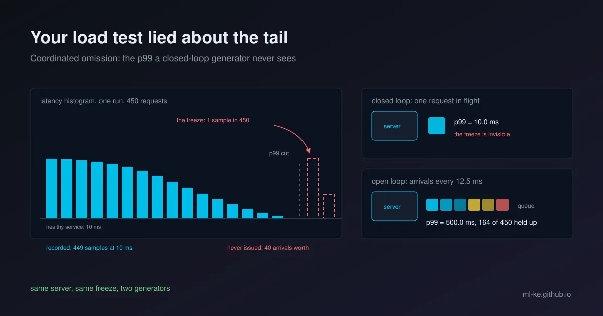
Same run, two answers: a p99 of 10 ms, and a service that stopped responding for half a second. This post builds that fixture in about forty lines of standard-library Python, shows the correction that recovers the samples the generator never took, and finishes with the utilization ceiling a p99 SLO actually buys you.
A p99 is the number a serving team puts in a launch review, an SLO document, or the capacity plan for the GPU it has to justify. It is also the easiest number in the report to get wrong, because the most common kind of load generator stops asking for work the moment the server stops answering, and the measurement then reports the good minutes while skipping the bad ones.
The generator waits in line with your users
Load generators come in two shapes. A closed-loop generator keeps a fixed number of requests in flight: send one, wait for the reply, send the next. An open-loop generator starts requests on a clock, whether or not earlier requests have finished. Grafana’s k6 documentation states the difference directly: in the closed model “the execution time of each iteration dictates the number of iterations executed in your test”, which is why k6 implements the open model in its arrival-rate executors. The same page names the failure mode. When slow responses produce fewer iterations, “in some testing literature, this problem is known as coordinated omission.”
Gil Tene coined the term in 2013 for percentile reports a closed-loop benchmark cannot be trusted to produce: the generator and the system under test coordinate, so the measurements that would have been taken during a stall are never taken. The ecosystem moved. k6 documents its constant-arrival-rate executor as open-model, starting iterations “independently of system response”, and NVIDIA’s Perf Analyzer splits the idea across two flags, a concurrency mode that keeps N requests outstanding and a request-rate mode that sends N requests per second.
The distinction bites at the tail. A closed loop with one virtual user records a stall once, because the single request in flight is the only one that can be slow. Real traffic does not wait its turn: requests keep arriving during the freeze and queue behind it.
Reproducing the lie
The fixture is small on purpose: a server whose healthy service time is 10 ms, one 500 ms freeze starting at t = 1 s (a stop-the-world pause, a model reload, a downstream that went away and came back), and a test that intends to issue 80 requests per second, one arrival every 12.5 ms.
1
2
3
4
5
6
7
8
9
10
11
12
13
14
15
16
17
18
19
20
21
22
23
24
25
26
27
28
29
30
31
32
33
34
35
36
37
38
39
40
41
42
43
44
45
46
47
48
49
50
51
52
53
54
55
56
57
58
59
60
61
62
63
64
65
66
67
68
69
70
71
72
73
74
75
def finish(begin, service, stall):
    """Completion time for a request that starts service at `begin`, on a server
    that makes no progress between stall[0] and stall[1] (GC pause, model reload,
    a downstream that went away)."""
    end = begin + service
    if end <= stall[0] or begin >= stall[1]:
        return end
    done = max(0.0, stall[0] - begin)         # work that got through before the freeze
    return stall[1] + (service - done)


def closed_loop(n=450, service=10.0, think=2.5, stall=(1000.0, 1500.0)):
    """One virtual user: send, wait for the reply, think, send again."""
    sends, ends, prev_end = [], [], 0.0
    for _ in range(n):
        send = prev_end + think
        ends.append(finish(max(send, prev_end), service, stall))
        sends.append(send)
        prev_end = ends[-1]
    return sends, ends


def open_loop(n=450, interval=12.5, service=10.0, stall=(1000.0, 1500.0)):
    """A steady arrival stream: a new request starts every `interval` ms whether
    or not the previous one has finished (an open-loop load generator)."""
    arrivals, ends, prev_end = [], [], 0.0
    for i in range(n):
        t = i * interval
        ends.append(finish(max(t, prev_end), service, stall))
        arrivals.append(t)
        prev_end = ends[-1]
    return arrivals, ends


def fill_in_corrected(samples, interval):
    """Gil Tene's correction: for every sample you recorded, add the samples the
    generator never issued because it was waiting (one per missed `interval`)."""
    out = []
    for v in samples:
        while v > interval:
            out.append(v)
            v -= interval
        out.append(v)
    return out


def pct(xs, p):
    xs = sorted(xs)
    return xs[min(len(xs) - 1, int(round(p / 100 * (len(xs) - 1))))]


INTERVAL = 12.5                      # the test's declared intent: 80 requests/s
FREEZE = 500.0

sends, ends = closed_loop()
raw = [e - s for s, e in zip(sends, ends)]
filled = fill_in_corrected(raw, INTERVAL)
lagging = [e - i * INTERVAL for i, e in enumerate(ends)]          # the naive variant

arr, oends = open_loop()
openloop = [e - a for a, e in zip(arr, oends)]

for name, series in (("closed loop raw      ", raw),
                     ("closed loop corrected", filled),
                     ("closed loop, lagged  ", lagging),
                     ("open loop (80 req/s) ", openloop)):
    print(f"{name} n={len(series):3d}  p50={pct(series,50):6.1f}  p90={pct(series,90):6.1f}  "
          f"p99={pct(series,99):6.1f}  max={max(series):6.1f}  >100ms={sum(1 for x in series if x > 100):3d}")

service_rate = 1000 / 10.0           # requests/s the server retires
arrival_rate = 1000 / INTERVAL       # requests/s arriving
backlog = FREEZE / INTERVAL
print(f"\nfreeze {FREEZE:.0f} ms -> {backlog:.0f} arrivals had to happen anyway; "
      f"queue clears in {backlog / (service_rate - arrival_rate):.1f} s "
      f"at {arrival_rate / service_rate:.0%} utilization")
1
2
3
4
5
6
closed loop raw       n=450  p50=  10.0  p90=  10.0  p99=  10.0  max= 507.5  >100ms=  1
closed loop corrected n=490  p50=  10.0  p90=  10.0  p99= 445.0  max= 507.5  >100ms= 33
closed loop, lagged   n=450  p50= 510.0  p90= 510.0  p99= 510.0  max= 510.0  >100ms=370
open loop (80 req/s)  n=450  p50=  10.0  p90= 397.5  p99= 500.0  max= 510.0  >100ms=164

freeze 500 ms -> 40 arrivals had to happen anyway; queue clears in 2.0 s at 80% utilization
The first row is the lie in textbook form. The service froze for half a second and the headline percentile does not move: p99 = 10.0 ms. One slow sample out of 450 sits above the p99 cut (1/450 is 0.22%, and the percentile only needs to exclude 1%), so the freeze is present in the data and absent from the statistics. The maximum, 507.5 ms, is the only hint left on a dashboard.
The second row applies the correction: 450 recorded samples become 490, the p99 moves to 445.0 ms, and 33 samples sit above 100 ms. The mechanism is fill_in_corrected above: every sample larger than the expected interval expands into the samples the generator would have taken in that time, one per missed 12.5 ms slot. That is how HdrHistogram’s correction works in practice.
The third row is the variant most people write first, and it fails. Subtracting the intended start time from each completion gives a p50 of 510 ms, because a single-threaded generator never recovers the slots it lost during the freeze; every later request stays half a second behind the schedule it declared, and 370 of 450 samples land above 100 ms. It claims the service was slow for five more seconds. It was not.
The fourth row is the honest measurement. With arrivals on a 12.5 ms clock, p99 is 500.0 ms and 164 of 450 requests (36%) were held up, because the freeze deposited a queue that then had to drain. The arithmetic at the end of the output says how long: 500 ms of arrivals is 40 requests of backlog, the server retires 100 requests/s against 80 arriving, so the queue drains at 20 requests/s and the last victim finishes 2.0 s after the freeze began. A half-second pause costs two seconds of tail, and only the open-loop run shows the whole bill.
What a correction can and cannot recover
The corrected figure (445 ms) and the measured open-loop figure (500 ms) are 12% apart, and the gap is the useful part. A correction reconstructs the samples a declared rate implies. It does not measure what happened, and it depends on a number you supplied.
HdrHistogram, whose API the correction is usually implemented through, describes recordValueWithExpectedInterval() as recording “an appropriate number of additional values” when a sample exceeds the expected interval, producing data “that would much more accurately reflect the response time distribution that a random, uncoordinated request would have experienced”. YCSB 0.2.0 RC1 adopted that measurement, and Friedrich, Wingerath and Ritter then built an open-system benchmark (NoSQLMark) to compare the two. Their Cassandra experiment ran a 1,000 ops/s target with a one-second hiccup simulated after 30 seconds and found that “even if the number of threads increases further, the intended values are higher than those of NoSQLMark… particularly… the mean value and the 90-percentiles”.
So a corrected percentile is a bound. In their setup it erred high; in the fixture above it erred low. Prefer an open-loop generator when you control the test, keep the correction for closed-loop runs you already have, and label which one produced a number before comparing it with anything.
Utilization is the budget, not a dial
The reason a 500 ms freeze costs two seconds of tail is queueing, and queueing has a closed form worth memorizing. For a single server with Poisson arrivals at rate $\lambda$ and exponential service at mean $1/\mu$, utilization is $\rho = \lambda/\mu$ and the queue is stable only while $\rho < 1$. Mean sojourn time (wait plus service) is $1/(\mu - \lambda)$. The distribution is tidier than it has any right to be: the sojourn time is exponential with parameter $\mu(1-\rho)$, so the chance a request waits longer than $a$ times the mean is $e^{-a}$.
Set the survival probability to 1% and solve:
\[e^{-a} = 0.01 \quad\Longrightarrow\quad a = \ln 100 = 4.605 \quad\Longrightarrow\quad \mathrm{p99} = \frac{4.605}{1-\rho} \text{ mean service times}\]That line is the capacity argument: the tail of a shared server is a function of how close to saturation you run it, and it is indifferent to your model, your framework and your prompt design.
1
2
3
4
5
6
7
8
9
10
11
12
13
14
15
16
17
18
19
20
21
22
23
24
25
26
27
28
29
30
31
32
33
34
35
36
37
import math
import random
import statistics


def mm1(rho, n, seed=7):
    """M/M/1 in service-time units: arrivals at rate rho, one server at rate 1."""
    rng = random.Random(seed)
    t = prev_end = 0.0
    out = []
    for _ in range(n):
        t += rng.expovariate(rho)
        begin = max(t, prev_end)
        end = begin + rng.expovariate(1.0)
        out.append(end - t)
        prev_end = end
    return out


def pct(xs, p):
    xs = sorted(xs)
    return xs[min(len(xs) - 1, int(round(p / 100 * (len(xs) - 1))))]


N = 2_000_000
print(f"{'rho':>5} {'mean sim':>9} {'mean 1/(1-rho)':>15} {'p99 sim':>9} {'p99 ln(100)/(1-rho)':>20}")
detail = None
for rho in (0.50, 0.70, 0.80, 0.90, 0.95, 0.98):
    s = mm1(rho, N)
    if rho == 0.90:
        detail = s
    print(f"{rho:5.2f} {statistics.fmean(s):9.3f} {1/(1-rho):15.3f} "
          f"{pct(s,99):9.2f} {math.log(100)/(1-rho):20.2f}")

print(f"\nat rho=0.90: p50={pct(detail,50):.2f} p90={pct(detail,90):.2f} "
      f"p95={pct(detail,95):.2f} p99={pct(detail,99):.2f} p99.9={pct(detail,99.9):.2f} "
      f"max={max(detail):.1f} (mean service times)")
1
2
3
4
5
6
7
8
9
  rho  mean sim  mean 1/(1-rho)   p99 sim  p99 ln(100)/(1-rho)
 0.50     2.001           2.000      9.28                 9.21
 0.70     3.340           3.333     15.47                15.35
 0.80     5.016           5.000     23.26                23.03
 0.90    10.067          10.000     47.08                46.05
 0.95    20.404          20.000     92.22                92.10
 0.98    53.695          50.000    309.83               230.26

at rho=0.90: p50=6.94 p90=23.10 p95=30.22 p99=47.08 p99.9=77.62 max=139.7 (mean service times)
Two million arrivals per row, and the table is blunt about where the tail comes from. At 50% utilization the p99 is 9.2 mean service times; at 90% it is 46; at 95% it is 92. The mean moves in step (2.0, 10.0, 20.0), so the ratio of p99 to mean is a constant 4.6 at every level. Note the p50 at 90%: 6.94 service times, so the typical request is already waiting several service times before the tail begins.
The 0.98 row is the honest failure. The simulation reports a mean sojourn of 53.7 service times where the formula says 50.0, and a p99 of 309.8 against 230.3, because at that load the answer is dominated by a handful of long busy periods and two million samples no longer contain enough independent ones. It is also the row a capacity plan would most like to use.
One caveat. M/M/1 assumes exponential service times, and a batched GPU producing tokens is more predictable than that, so the real tail is usually better than the formula. The shape is the part that transfers: the p99 grows as $1/(1-\rho)$, the mean grows at the same rate, and the only term you control is $\rho$. The SRE book puts it operationally: load testing exists to “trade off utilization versus safety margins”.
Your p99 estimate carries its own error bar
The p99 is itself an estimate, and it converges slowly. Thirty independent 20,000-request tests at each load level, scored against the closed form:
1
2
3
4
5
6
7
8
9
10
11
12
13
14
15
16
17
18
19
20
21
22
23
24
25
26
27
28
29
import math
import random
import statistics


def mm1(rho, n, seed):
    """M/M/1 in service-time units. Returns the sojourn time of every arrival."""
    rng = random.Random(seed)
    t = prev_end = 0.0
    out = []
    for _ in range(n):
        t += rng.expovariate(rho)                 # Poisson arrivals at rate rho
        end = max(t, prev_end) + rng.expovariate(1.0)   # one server, unit mean
        out.append(end - t)
        prev_end = end
    return out


def pct(xs, p):
    xs = sorted(xs)
    return xs[min(len(xs) - 1, int(round(p / 100 * (len(xs) - 1))))]


print("30 independent 20,000-request load tests per utilization level")
print(f"{'rho':>5} {'theory p99':>11} {'median':>8} {'min':>7} {'max':>7} {'max/min':>8}")
for rho in (0.80, 0.90, 0.95):
    runs = [pct(mm1(rho, 20_000, seed), 99) for seed in range(30)]
    print(f"{rho:5.2f} {math.log(100)/(1-rho):11.2f} {statistics.median(runs):8.2f} "
          f"{min(runs):7.2f} {max(runs):7.2f} {max(runs)/min(runs):8.2f}")
1
2
3
4
5
30 independent 20,000-request load tests per utilization level
  rho  theory p99   median     min     max  max/min
 0.80       23.03    23.48   18.60   29.26     1.57
 0.90       46.05    44.46   30.18   71.49     2.37
 0.95       92.10    78.28   44.39  125.56     2.83
The medians land close to theory; the spread is the finding. At 80% utilization the worst of thirty runs is 1.6 times the best, at 90% it is 2.4 times, at 95% it is 2.8 times. A staging benchmark that makes 20,000 requests and reports a p99 of 50 ms cannot distinguish that result from 71 ms, and the same code reporting 30 ms on Monday and 60 ms on Friday has said nothing about your release. The reason is structural: long sojourns arrive in clusters inside long busy periods, so $n$ requests contain far fewer than $n$ independent observations of the tail, and fewer still as utilization rises.
That changes what you alarm on. Means and the fraction of requests over a fixed threshold converge quickly enough to gate a deploy. Percentiles need far more requests, several runs reported together, or a closed-form model to interpret them.
From an SLO to a utilization ceiling
The formula inverts, which turns a latency target into a capacity answer. If the p99 budget is $S$ times the mean service time, the highest utilization you can run at is $\rho_{\max} = 1 - \ln(100)/S$.
1
2
3
4
5
6
7
8
9
10
11
12
13
14
15
16
17
18
import math


def utilization_ceiling(p99_in_service_times):
    """Highest utilization an M/M/1 server can run at and still hold the 99th
    percentile sojourn time under `p99_in_service_times` mean service times."""
    return 1 - math.log(100) / p99_in_service_times


print(f"{'p99 SLO':>10} {'rho ceiling':>12} {'mean wait':>10} {'mean queue':>11}")
for slo in (5, 10, 20, 50, 100):
    rho = utilization_ceiling(slo)
    print(f"{slo:8d}x {rho:12.3f} {rho/(1-rho):9.2f}x {rho*rho/(1-rho):10.2f}x")

print("\nfan-out: each replica is slow on 1% of calls")
for m in (1, 10, 100):
    print(f"  {m:3d} replica(s): P(the request waits on a slow one) = {1 - 0.99**m:.4f}"
          f"   per-replica slow rate needed for 1% overall = {1 - 0.99**(1/m):.5f}")
1
2
3
4
5
6
7
8
9
10
11
   p99 SLO  rho ceiling  mean wait  mean queue
       5x        0.079      0.09x       0.01x
      10x        0.539      1.17x       0.63x
      20x        0.770      3.34x       2.57x
      50x        0.908      9.86x       8.95x
     100x        0.954     20.71x      19.76x

fan-out: each replica is slow on 1% of calls
    1 replica(s): P(the request waits on a slow one) = 0.0100   per-replica slow rate needed for 1% overall = 0.01000
   10 replica(s): P(the request waits on a slow one) = 0.0956   per-replica slow rate needed for 1% overall = 0.00100
  100 replica(s): P(the request waits on a slow one) = 0.6340   per-replica slow rate needed for 1% overall = 0.00010
Read the first column against your SLO. A p99 budget of ten mean service times permits 54% utilization, with a mean wait of 1.17 service times. Twenty times buys 77%. Fifty times, where many services actually run, means 91% utilization and a mean wait of 9.86 service times. No row appears for 98%, because 98% utilization is a statement that your p99 is unbounded rather than a plan.
The fan-out block covers the case where one user request is several requests. Dean and Barroso’s Tail at Scale example is the canonical version: a request that collects answers from 100 servers, each with a 1% chance of being slow, is slow with probability 63%. The table confirms the arithmetic (0.6340) and adds the constraint that follows. Holding the overall slow rate at 1% across 100 replicas needs a per-call slow rate of 0.0001 per replica, a p99.99 budget for each one, which is the price of sharding a retrieval index a hundred ways.
How to apply this to a model endpoint
| Step | Concrete check |
|---|---|
| Generate load on a clock | Use an arrival-rate executor (k6’s constant-arrival-rate, Perf Analyzer’s --request-rate-range, or a scheduler that fires independently of responses). A concurrency knob is a closed loop |
| Split the SLO before measuring | TTFT includes queueing and prefill, so it moves first under load; inter-token latency (TPOT) describes decoding. Budget them separately |
| Attribute the tail | vLLM exports queue intervals, TTFT and TPOT as histograms, so a p99 that breaks can be blamed on the queue rather than the model |
| Convert the SLO to a utilization ceiling | $\rho_{\max} = 1 - \ln(100)/S$ with $S$ in mean service times, then check the fleet at peak |
| Decide what to shed in advance | Utilization thresholds plus criticality let an overloaded service reject the work it can afford to lose instead of queueing everything |
| Re-run after every serving change | Quantization, a new batch cap and a new tokenizer all move the service-time distribution, so the same arrival rate yields a different p99 |
| Keep per-shard tail budgets | Fan-out multiplies the slow rate; a sharded index needs p99.99 per shard to look like p99 overall |
Two local notes. The same arithmetic governs a single-GPU deployment, the shape most teams on this blog actually run (see the constrained-environment and edge posts below): the p99 target sets the fraction of the card you can use, and the busy-hour arrival rate sets the number of replicas. Sizing on averages is how a one-card service ends up at 95% utilization with a tail it cannot explain. And the ceiling is not a licence to buy hardware for every spike: load shedding and a batch cap hold $\rho$ below it more cheaply than doubling the fleet.
Key takeaways
| Takeaway | Evidence in this post |
|---|---|
| A closed-loop generator hides a freeze at the tail | 500 ms freeze, closed loop: p99 10.0 ms, one sample above 100 ms |
| The correction fills in samples, not events | 450 recorded samples become 490; p99 445.0 ms, 33 above 100 ms |
| A naive intended-start correction inflates everything after the stall | p50 510.0 ms; 370 of 450 samples above 100 ms |
| The queue, not the pause, is the cost | 40 arrivals of backlog drain in 2.0 s at 80% utilization; 164 of 450 requests affected |
| The tail of a shared server is set by utilization | p99 = 4.605/(1-ρ) service times: 9.28 at ρ=0.50, 92.22 at ρ=0.95 |
| A sampled p99 is noisy, and noisier under load | 30 runs of 20,000 requests span 1.57x at ρ=0.80, 2.83x at ρ=0.95 |
| An SLO implies a utilization ceiling | 10x service time allows ρ ≤ 0.539; 20x allows ρ ≤ 0.770 |
| Fan-out multiplies the tail | 100 replicas at 1% slow each: 63% of requests slow; 0.01% per replica to hold 1% |
The fixture is synthetic and seeded, and every number above came out of the four blocks as published: the closed-loop experiment runs in milliseconds, the utilization table takes about twelve seconds because it generates two million arrivals per row. To point the harness at a real endpoint, replace the synthetic service time and freeze with measured per-request durations from an arrival-rate run. The two numbers worth keeping are the count of requests above the threshold and the sample size printed beside the percentile.
References
- Tene, G. (2013). How NOT to Measure Latency — ACM Queue; the talk that named coordinated omission.
- Grafana Labs. Open and closed models — k6 docs; the closed model couples iteration rate to response time.
- Grafana Labs. Constant arrival rate — the open-model executor.
- HdrHistogram. README —
recordValueWithExpectedInterval()and corrected-versus-raw recording. - Friedrich, S., Wingerath, W., Ritter, N. (2017). Coordinated Omission in NoSQL Database Benchmarking — BTW 2017; intended-interval correction measured against an open-system benchmark.
- Wikipedia contributors. M/M/1 queue — ρ = λ/μ, stability, and the mean sojourn time 1/(μ − λ).
- van der Mei, R. The M/M/1 queue — lecture notes; sojourn time is exponential with parameter μ(1−ρ), hence P(S > aE(S)) = e^{−a}.
- Dean, J., Barroso, L. A. (2013). The Tail at Scale — CACM 56(2); the 100-server, 63% fan-out example.
- Beyer, B., Jones, C., Petoff, J., Murphy, N. R. (eds.). SRE, ch. 21: Handling Overload — utilization thresholds, criticality and shedable work.
- Beyer, B., Jones, C., Petoff, J., Murphy, N. R. (eds.). SRE, ch. 22: Addressing Cascading Failures — load test until components break; utilization versus safety margin.
- NVIDIA. Perf Analyzer: inference load modes — concurrency mode versus request-rate mode.
- NVIDIA. LLM benchmarking metrics — TTFT includes queueing, prefill and network; ITL is time per output token.
- Anyscale. Understand LLM latency and throughput metrics — end-to-end latency is TTFT plus generation time.
- vLLM project. Metrics — queue intervals, TTFT and TPOT as histograms.
- Varadarajan, B. (2026). The LLM Inference Trilemma: Throughput, Latency, Cost — TTFT and ITL SLOs at p50/p95/p99.
Related posts
- vLLM and High-Throughput LLM Serving: PagedAttention and Continuous Batching — the batching behaviour that sets the service-time distribution you are measuring.
- Half the Cache, Twice the Context: measuring what KV quantization costs at long range — the other half of a latency budget, measured rather than assumed.
- Guess Ahead, Pay Once: Speculative Decoding You Can Verify — where a speedup claim survives verification and where it does not.
- Building and Deploying AI in Constrained Environments: Low-Bandwidth and Edge Solutions — the single-node deployments where utilization ceilings decide the hardware list.
- Paging the Ledger: Real-Time Reconciliation Alerting That Actually Wakes Someone — alerting on the numbers that converge, rather than the ones that do not.