44,000 Seeds, One Open Map: What the Dryland Sorghum Pangenome Changes for Breeders

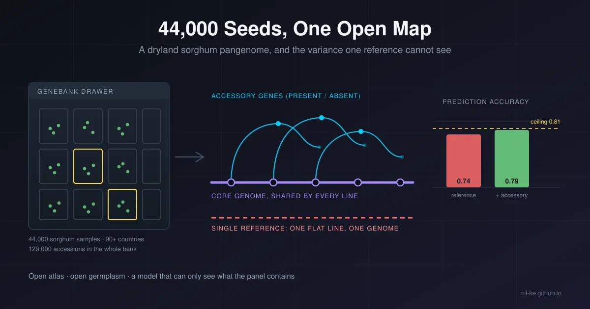
In one paragraph: On 15 October 2026 Google DeepMind and Google.org said they will build an open-access genetic atlas for sorghum with ICRISAT, the HudsonAlpha Institute for Biotechnology and the University of Washington, sampling a genebank that holds more than 44,000 sorghum collections from over 90 countries. DeepMind is also funding a three-year postdoctoral fellowship at ICRISAT, its first in India and its first outside the UK. No dataset, licence or release date came with the announcement, so the useful question is not what shipped, because nothing did. It is what the design makes possible, and what a breeding programme can measure today.

Two other releases sit close enough to be mistaken for this one. The AlphaGenome variant atlas is a human-genetics resource: prefetch a variant, score it, rank it. September’s Gates and Google farmer stack was advisory: put a recommendation in a smallholder’s hand. This announcement is neither. It is the map underneath both, the layer a breeder reads years before anything reaches a farmer, and it comes with DeepMind’s first research fellowship outside the UK attached to a crop that African drylands eat.

What was announced, and by whom

The release is short and specific about partners, vaguer about deliverables. Google DeepMind brings machine learning and a fellowship. Google.org brings money through the AI Collaborative for Food Security, the same vehicle behind September’s advisory push. ICRISAT brings the germplasm: a genebank of more than 129,000 accessions across 11 crops, built from collection missions in 144 countries, 80.8% of it landraces. The new work draws a representative sample of “over 44,000 genetic samples from over 90 countries” from that collection.

Partner	Stated role	Detail worth keeping
Google DeepMind	machine learning, plus a three-year postdoctoral fellowship at ICRISAT	first DeepMind fellowship in India and first outside the UK
Google.org, via the AI Collaborative for Food Security	funds the collaboration	same collaborative as the September advisory announcement
ICRISAT	germplasm and breeding science, Hyderabad headquarters	genebank holds >129,000 accessions; regional genebanks in Niamey, Bulawayo and Nairobi
HudsonAlpha Institute for Biotechnology	research partner	named in the release alongside ICRISAT and UW
University of Washington, Dept. of Genome Sciences	research partner	named in the release

What the partners describe building is an “open-access Global Public Good”: a genetic atlas of indigenous sorghum collections that pairs “advanced genetic analysis with machine learning to identify the most promising plant combinations”. Google DeepMind’s food-security portfolio lead, Abi Ramanan, calls it “the first Global Dryland Sorghum Pangenome” and describes sorghum as a crop that “sustains the nutrition of over 500 million of the world’s most climate-vulnerable people”. The fellowship is scoped beyond sorghum, to build the same kind of characterisation for chickpea, groundnut and pigeon pea.

Two sentences in that release are load-bearing, and both are claims rather than results. “First” is a marketing word until someone checks the citation, and “open-access” is a promise until a licence file exists. What is not in doubt is the input: 44,000 accessions is roughly a third of the whole genebank, and the best public sorghum pangenome to date rests on 33 assembled genomes.

Why sorghum earns a pangenome first

Sorghum is the crop you breed when rain is a rumour. It is also, by the numbers, the crop where the distance between what the land yields and what the crop can yield costs the most grain.

Measure	Value	Source
Sorghum area in sub-Saharan Africa, 31 countries, 2001 to 2020 average	~24.5 million ha	FAOSTAT-derived analysis, Frontiers 2023
Share of that area in six countries (Nigeria, Sudan, Niger, Ethiopia, Mali, Burkina Faso)	70.6%, roughly 17.3 million ha	same
Sub-Saharan Africa average yield	~0.9 t/ha	same
Global average yield, 2001 to 2020	2.5 t/ha	same
Global harvested area, 1961-80, 1981-2000, 2001-20	46.3, 43.2, 40.9 million ha	same

A 2.8x yield gap on 24.5 million hectares is the arithmetic that justifies everything downstream. Lifting sub-Saharan Africa from 0.9 to 1.5 t/ha on that area is 14.7 million tonnes of grain; reaching the global average would be 39.2 million. Note the direction of the historical trend too: sorghum’s global production gains since 1961 came from yield, not from clearing more land, while harvested area fell 11.7%. There is no new land in this story. There is only better seed.

Breeding better seed for those six countries means breeding against drought, Striga and aluminium toxicity, and breeding for the low-input conditions most of its growers farm in. Every one of those traits is genetic, and every one of them is unevenly distributed across a species that diverged into distinct gene pools.

One reference genome, and what it edits out

Modern genomics runs on a single reference. For sorghum that has been BTx623, a line chosen for practical reasons, not because it represents the species. Reads from a Malian landrace or a Sudanese striga-resistant line get mapped onto BTx623, and anything that line does not contain either fails to map or gets squeezed into a gap.

That is fine for single-letter differences and bad for the variation breeders care about. The March 2026 sorghum pangenome in Nature, from a consortium including the Danforth Center, HudsonAlpha, the Joint Genome Institute and several universities, put the problem in one sentence: large-scale structural variants, copy-number variants and presence-absence variants are “often not perfectly captured by short reads mapped to a single reference genome”. Its fix was 33 assembled genomes, including the transformable RTx430, the stay-green BTx642, sweet Wray and 20 cultivars the breeding community actually uses, plus whole-genome resequencing of 1,984 cultivars and landraces. The panel covers 693 unique African and Asian cultivars with georeferenced collection locations, and includes lines such as SRN39 from Sudan for striga resistance, SC 283 for aluminium tolerance and CSM-63 for water-use efficiency.

The new project takes that method from 33 genomes to a 44,000-accession question. That is the interesting shift: not a better model, a bigger and more representative panel behind it.

What a model can see, measured

Here is the part a breeding programme can test this week, without waiting for the atlas. The claim underneath every pangenome argument is that a reference-only view caps prediction accuracy, because a gene the panel cannot see contributes variance the model cannot attribute. That claim is measurable in a simulation small enough to run on a laptop.

I built a synthetic genebank panel with three landrace groups, 400 core SNP markers standing in for single-reference genotypes, and 36 accessory genes present or absent in a way that depends on the group. Twenty core markers and eight accessory genes are causal, and the accessory effects are scaled so the accessory genome carries about a third of the genetic variance. The true breeding value is known by construction, phenotype heritability is 0.7, and everything is seeded.

import numpy as np

def build_panel(seed=7, n_per_pop=200, n_core=400, n_pav=36,
                n_causal_core=20, n_causal_pav=8, pav_share=0.35, h2=0.7):
    rng = np.random.default_rng(seed)
    pops = np.repeat([0, 1, 2], n_per_pop)               # three landrace groups
    n = pops.size
    freqs = rng.uniform(0.08, 0.92, size=(3, n_core))
    core = np.empty((n, n_core), dtype=np.int8)          # SNP dosages: one reference view
    for i, p in enumerate(pops):
        core[i] = rng.binomial(2, freqs[p])
    pav_rate = np.array([0.15, 0.40, 0.75])              # accessory genes: present/absent
    pav = (rng.random((n, n_pav)) < pav_rate[pops][:, None]).astype(np.int8)
    b_core = np.zeros(n_core)
    b_core[rng.choice(n_core, n_causal_core, replace=False)] = rng.normal(0, 1, n_causal_core)
    b_pav = np.zeros(n_pav)
    b_pav[rng.choice(n_pav, n_causal_pav, replace=False)] = rng.normal(0, 1, n_causal_pav)
    core_part, pav_part = core @ b_core, pav @ b_pav
    b_pav *= np.sqrt(pav_share / (1 - pav_share) * core_part.var() / pav_part.var())
    pav_part = pav @ b_pav
    g = core_part + pav_part
    g = (g - g.mean()) / g.std()                         # true breeding value
    y = g + rng.normal(0, np.sqrt((1 - h2) / h2), n)      # what a field trial measures
    return dict(core=core, pav=pav, g=g, y=y, pops=pops,
                core_part=core_part, pav_part=pav_part)

P = build_panel()
share = np.var(P["pav_part"]) / np.var(P["pav_part"] + P["core_part"])
print("accessions: %d | landrace groups: %d" % (P["g"].size, len(np.unique(P["pops"]))))
print("core SNP markers: %d | accessory genes: %d" % (P["core"].shape[1], P["pav"].shape[1]))
print("accessory-genome share of genetic variance: %.1f%%" % (100 * share))
print("ceiling for a panel that cannot see them: r = %.3f" % np.sqrt(1 - share))

accessions: 600 | landrace groups: 3
core SNP markers: 400 | accessory genes: 36
accessory-genome share of genetic variance: 33.9%
ceiling for a panel that cannot see them: r = 0.813

That last line is just arithmetic, and it is the one to remember. If 33.9% of genetic variance sits in genes the reference view cannot observe, then a reference-only model’s correlation with the true breeding value cannot exceed the square root of the remaining 66.1%, which is 0.813, no matter how much data you feed it.

The second block fits the same panel twice with ridge regression, which is algebraically the same as GBLUP when the marker matrix is centered and scaled. Once with the 400 core markers, once with core plus the 36 accessory genes, scored against the known true breeding value, under two validation schemes.

import numpy as np

def build_panel(seed=7, n_per_pop=200, n_core=400, n_pav=36,
                n_causal_core=20, n_causal_pav=8, pav_share=0.35, h2=0.7):
    rng = np.random.default_rng(seed)
    pops = np.repeat([0, 1, 2], n_per_pop)
    n = pops.size
    freqs = rng.uniform(0.08, 0.92, size=(3, n_core))
    core = np.empty((n, n_core), dtype=np.int8)
    for i, p in enumerate(pops):
        core[i] = rng.binomial(2, freqs[p])
    pav_rate = np.array([0.15, 0.40, 0.75])
    pav = (rng.random((n, n_pav)) < pav_rate[pops][:, None]).astype(np.int8)
    b_core = np.zeros(n_core)
    b_core[rng.choice(n_core, n_causal_core, replace=False)] = rng.normal(0, 1, n_causal_core)
    b_pav = np.zeros(n_pav)
    b_pav[rng.choice(n_pav, n_causal_pav, replace=False)] = rng.normal(0, 1, n_causal_pav)
    core_part, pav_part = core @ b_core, pav @ b_pav
    b_pav *= np.sqrt(pav_share / (1 - pav_share) * core_part.var() / pav_part.var())
    g = core_part + pav @ b_pav
    g = (g - g.mean()) / g.std()
    y = g + rng.normal(0, np.sqrt((1 - h2) / h2), n)
    return core, pav, g, y, pops

def fit(X, y, lam):
    mu, sd = X.mean(0), X.std(0)
    sd[sd == 0] = 1.0
    Xs = (X - mu) / sd
    ym = y.mean()
    w = np.linalg.solve(Xs.T @ Xs + lam * np.eye(Xs.shape[1]), Xs.T @ (y - ym))
    return w, mu, sd, ym

def predict(model, X):
    w, mu, sd, ym = model
    return ((X - mu) / sd) @ w + ym

LAMS = [3.0, 30.0, 300.0]

def pick_lambda(X, y, seed=0):
    idx = np.random.default_rng(seed).permutation(len(y))
    cut = int(0.8 * len(y))
    tr, va = idx[:cut], idx[cut:]
    best, best_mse = LAMS[0], np.inf
    for lam in LAMS:
        mse = np.mean((predict(fit(X[tr], y[tr], lam), X[va]) - y[va]) ** 2)
        if mse < best_mse:
            best, best_mse = lam, mse
    return best

def split_cv(X, y, g, groups=None, folds=5, seed=1):
    """Random folds, or leave one landrace group out when groups is given."""
    if groups is None:
        parts = np.array_split(np.random.default_rng(seed).permutation(len(y)), folds)
        sets = [(np.concatenate([parts[j] for j in range(folds) if j != k]), parts[k])
                for k in range(folds)]
    else:
        sets = [(groups != u, groups == u) for u in np.unique(groups)]
    pred = np.empty_like(y)
    for tr, te in sets:
        lam = pick_lambda(X[tr], y[tr])
        pred[te] = predict(fit(X[tr], y[tr], lam), X[te])
    return np.corrcoef(pred, g)[0, 1]

def holdout(X, y, g, n_train, seed=2):
    idx = np.random.default_rng(seed).permutation(len(y))
    tr, te = idx[:n_train], idx[n_train:]
    pred = predict(fit(X[tr], y[tr], pick_lambda(X[tr], y[tr])), X[te])
    return np.corrcoef(pred, g[te])[0, 1]

core, pav, g, y, pops = build_panel()
X_ref, X_pan = core, np.hstack([core, pav])

print("accuracy = correlation between the predicted value and the TRUE breeding value")
print()
print("random 5-fold cross-validation, 600 accessions")
print("  reference panel only (400 SNPs)  r = %.3f" % split_cv(X_ref, y, g))
print("  plus accessory genome (36 genes) r = %.3f" % split_cv(X_pan, y, g))
print()
print("leave-one-landrace-group-out (train on two groups, predict the third)")
print("  reference panel only             r = %.3f" % split_cv(X_ref, y, g, pops))
print("  plus accessory genome            r = %.3f" % split_cv(X_pan, y, g, pops))
print()
print("training-set size sweep, single holdout")
for n in (60, 120, 240, 460):
    print("  n_train=%3d  reference r = %.3f  pangenome r = %.3f"
          % (n, holdout(X_ref, y, g, n), holdout(X_pan, y, g, n)))

accuracy = correlation between the predicted value and the TRUE breeding value

random 5-fold cross-validation, 600 accessions
  reference panel only (400 SNPs)  r = 0.738
  plus accessory genome (36 genes) r = 0.793

leave-one-landrace-group-out (train on two groups, predict the third)
  reference panel only             r = 0.294
  plus accessory genome            r = 0.625

training-set size sweep, single holdout
  n_train= 60  reference r = 0.540  pangenome r = 0.583
  n_train=120  reference r = 0.560  pangenome r = 0.565
  n_train=240  reference r = 0.696  pangenome r = 0.744
  n_train=460  reference r = 0.755  pangenome r = 0.815

Three things in that output matter, and none of them is specific to sorghum.

The gap under random folds is 0.055: 0.738 with the reference view, 0.793 with the accessory genes added. Neither number is a claim about real sorghum, and the 0.738 sits below the 0.813 ceiling because finite training data and shrinkage both cost accuracy. The structural point stands. The model that cannot see a third of the variance cannot reach the ceiling that variance implies.

The second block is the one that should change how a breeder reads a validation table. Under random folds, every test line has siblings in the training set, so accuracy is measured on relatives. Hold out an entire landrace group and the reference panel collapses from 0.738 to 0.294, while the pangenome model falls from 0.793 to 0.625. Both get worse. Only one survives a new environment with unfamiliar germplasm, which is the actual deployment condition for a breeding programme in a country it has never collected in.

The third block is a warning about single numbers. Accuracy rises with training-set size in both views, from 0.540 and 0.583 at 60 lines to 0.755 and 0.815 at 460, but the gap between the two views wanders: 0.043, 0.005, 0.048, 0.060. One holdout draw is noisy. Any breeder publishing a single accuracy figure from a single split is publishing noise with a decimal point.

Where the machine learning actually sits

It is worth being precise about which parts of a 44,000-accession pangenome are ML problems, because the announcement’s framing (“machine learning to identify the most promising plant combinations”) blurs them.

• Assembly and presence-absence calling at scale. Deciding whether a gene is missing from a line or merely unassembled is a graph and coverage problem, and it is the step most likely to be wrong. A pangenome graph that mis-calls PAVs produces confident predictions about genes that do not exist.
• Imputation from cheap genotyping. If a programme can skim-sequence a line at low coverage and impute the rest against a pangenome, the cost per genotyped plant falls sharply. That is the biggest practical lever in the whole project, and it is a statistical model, not a neural network.
• Genomic prediction. Ridge regression or GBLUP, as in the demo. Well understood, cheap, and adequate for additive traits when the training population is designed properly.
• Genotype-by-environment modelling. This is where most field failures live. A model that predicts performance in the trial site and not in the farmer’s field has learned the site.
• The fellowship’s actual job. Porting the pipeline to chickpea, groundnut and pigeon pea is three more genebanks’ worth of assembly, imputation and phenotype curation. Naming it in the release is the most credible sentence in the document, because it is the part that takes years.

The pattern to keep in view: the atlas is the contribution. The model on top of it is the easy part, and every one of these steps degrades to noise if phenotype records are thin.

How a breeding programme uses it next season

Nothing in the list below requires the new atlas. It requires a training population that spans diversity, honest validation, and phenotype data good enough to fit anything at all.

Step	Artifact you need	The test that can fail
1. Choose a training set that spans groups and environments	passport data, georeferenced origins	hold out one group and check accuracy before trusting the set
2. Phenotype with replication and record the environment	plot-level records, weather, soil	repeatability across years, not a single season
3. Genotype cheaply and impute against a pangenome	low-coverage sequence, imputation panel	imputation accuracy per group, not pooled
4. Fit a small model	ridge or GBLUP on centered, scaled markers	accuracy against the true value, not against phenotype
5. Validate by group and by year	a split the model has never seen	random-fold accuracy is the number to distrust
6. Report against a ceiling	the variance your markers can actually see	a score above the ceiling means leakage, not genius

Step five is the one the demo earns. Random cross-validation answers “can the model rank siblings”, which is not the question a breeder asks. Group-wise validation answers “does this transfer to germplasm from a place I have not sampled”, which is.

Three caveats worth writing down

The first is that this is a plan. There is no atlas to download, no licence text, no deposit and no date in the release. Everything about openness is a stated intention until the first dataset lands, and the licence matters more than the press release: a pangenome that is readable but not reusable is a poster.

The second is that the germplasm was never the closed part. ICRISAT already distributes seed free, has repatriated 55,399 accessions to 11 national programmes and has sent 1.61 million seed samples to researchers in 150 countries. What the project adds is the sequence and assembly layer on top, which is exactly the layer where access terms usually get restrictive.

The third is that prediction is not yield. A genomic model estimates a breeding value in a defined population and environment; a farmer harvests a crop under striga pressure, mid-season dry spells and little fertiliser. Every number in this post comes from a simulation I built to isolate one mechanism, and it proves arithmetic, not agronomy.

Key takeaways

Point	Detail
What was announced	Google DeepMind, Google.org, ICRISAT, HudsonAlpha and UW will build an open-access sorghum genetic atlas from a representative sample of >44,000 genebank accessions, plus a three-year fellowship at ICRISAT
Why it matters	sub-Saharan Africa grows sorghum on ~24.5 million ha at ~0.9 t/ha against a 2.5 t/ha global average, and gains have to come from seed, not land
The technical bet	a single reference genome cannot see presence-absence and structural variation, so a reference-only panel caps prediction accuracy at the square root of the variance it can observe
Measured gap	in a seeded simulation, random-fold accuracy 0.738 reference-only against 0.793 with accessory genes; holding out a whole landrace group drops the reference model to 0.294 against 0.625
The rule to steal	validate across groups and years, never across random rows, and report accuracy against the variance your markers can see

References

• ICRISAT, From lab to impact: Advancing AI for real-world progress in India (release adapted from the Google blog, 16 October 2026) — ICRISAT pressroom
• Google DeepMind, ICRISAT Partner to Advance AI-Driven Crop Research — Global Agriculture, 16 October 2026
• Google DeepMind ties up with ICRISAT to develop plant genome atlas — Business Standard, 15 October 2026
• ICRISAT, Genebank: about (129,000 accessions, 144 countries, 80.8% landraces, regional genebanks) — icrisat.org
• Morris, Harder, Healey et al., A sorghum pangenome reference improves global crop trait discovery — Nature, 11 March 2026
• Danforth Plant Science Center, Global sorghum pangenome accelerates discovery of resilient crop traits (33 genomes, 1,984 resequenced lines) — phys.org, 12 March 2026
• Khalifa & Eltahir, Assessment of global sorghum production, tolerance, and climate risk (FAOSTAT area, yield and yield-gap figures) — Frontiers in Sustainable Food Systems, 2023
• Training Population Optimization for Genomic Selection (drivers of predictive ability: phenotype quality, marker coverage, training-set size and relatedness) — PMC, 2019
• Genomic selection in plant breeding: key factors shaping two decades of progress — Molecular Plant, 2024

Related posts

• The Farmer, the Model, and the 200 Million: Reading Google and Gates’ Advisory Stack — the advisory layer this atlas sits underneath
• Nine Billion Variants, One Atlas: What DeepMind’s AlphaGenome Atlas Makes Testable — the same atlas pattern applied to human variation
• AI for Agriculture: Where the Models Actually Pay Off — disease detection and yield prediction, one layer up from the genome
• Africa’s Agriculture Is a Climate Problem Before It Is an AI Problem — the climate and input constraints that decide whether a better variety helps