Is Your +3-Point Eval Gain Real? Gating a Comparison with Paired Statistics

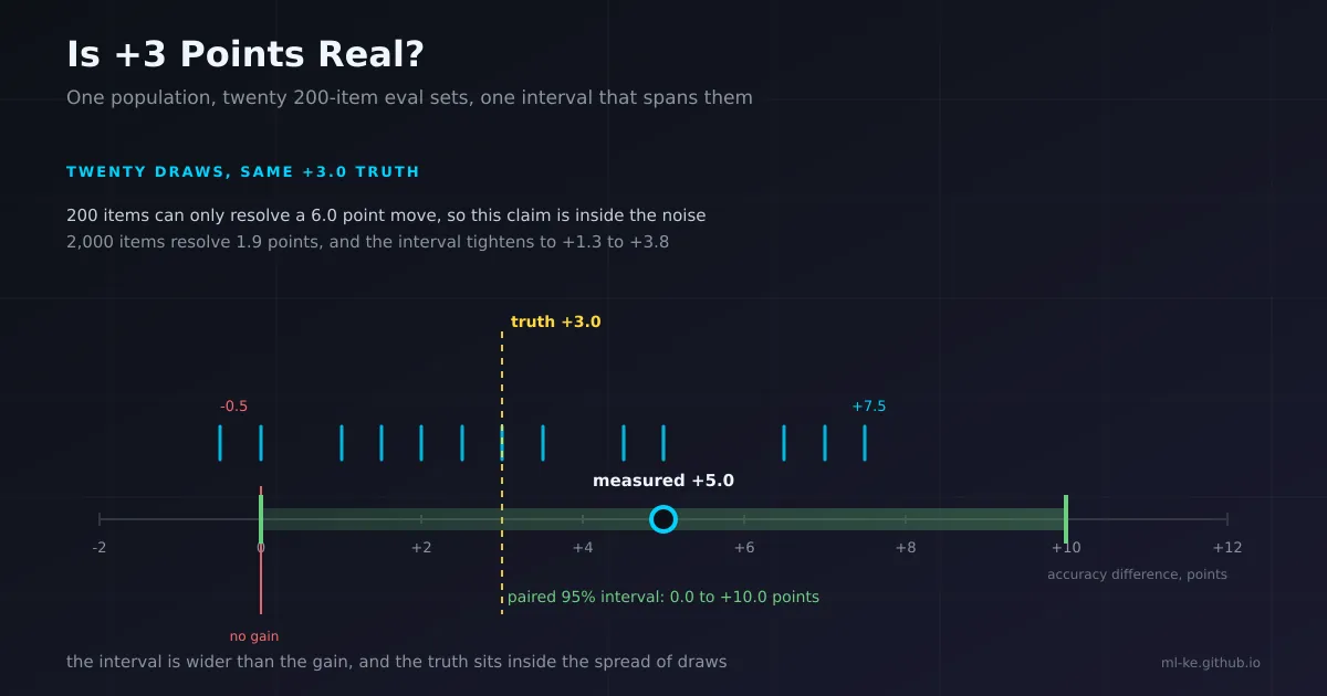
The short version “The new prompt is 3.2 points better on our eval” is the most common performance claim in applied ML, and one of the least often tested. This post builds an eval set whose true difference is +3.0 points by construction, then runs the four checks that decide whether a measured gain survives its own sampling error: the per-item pairing table, McNemar’s test on the discordant pairs, a paired bootstrap interval on the delta, and the sample size needed to detect the effect you claim. The final experiment finds the items that flip when you re-run.

Every model changelog has the sentence. The number is a difference of two accuracies, reported to one decimal place, with no interval and no mention of how many items the eval contained.

The fixture below is synthetic on purpose, because synthetic is the only way to know the truth: the population difference is fixed at +3.0 points, so every estimate can be scored against what it recovers. Your own per-item results change none of the arithmetic.

Four recent posts in this lane measure one system against a fixed reference: calibration on whether a probability means what it says, annotator agreement on whether two people agree on a label, recall at k on whether the right document reached the top of a list, and the load test post on whether p99 was measured honestly. None compares two systems on the same items, which is the comparison with its own arithmetic and its own failure mode.

A gain is a difference between two columns

The fixture draws each item’s easiness between zero and one, then scores it for both systems. A system passes an item when its noisy read of that easiness clears that system’s bar, and the new prompt’s bar sits three points lower. That is a serviceable model of a prompt change that fixes a class of near misses: identical on the easy items, identical on the hopeless ones, different near the boundary where most of the argument lives.

import math, random

T_A, T_B = 0.60, 0.63      # an item passes when its easiness clears the system's bar
NOISE = 0.08               # per-run wobble: the same item, scored twice

def build(n, seed):
    rng = random.Random(seed)
    rows = []
    for _ in range(n):
        e = rng.random()                                  # how easy this item is
        a = 1 if e + NOISE * rng.gauss(0, 1) < T_A else 0
        b = 1 if e + NOISE * rng.gauss(0, 1) < T_B else 0
        rows.append((e, a, b))
    return rows

def summarise(rows):
    n = len(rows)
    a = sum(r[1] for r in rows) / n
    b = sum(r[2] for r in rows) / n
    only_b = sum(1 for r in rows if r[1] == 0 and r[2] == 1)
    only_a = sum(1 for r in rows if r[1] == 1 and r[2] == 0)
    return n, a, b, b - a, only_b, only_a, 1 - (only_b + only_a) / n

pop = summarise(build(200_000, 7))
print(f"population truth, 200,000 items: A {pop[1]:.3f}  B {pop[2]:.3f}  delta {pop[3]:+.3f}")

print(f"\n{'set':10s}{'n':>6s}{'A':>7s}{'B':>7s}{'delta':>8s}{'b':>5s}{'c':>5s}{'agree':>8s}")
for name, n, seed in (("eval-200", 200, 20261266), ("eval-2000", 2000, 20261022)):
    s = summarise(build(n, seed))
    print(f"{name:10s}{s[0]:6d}{s[1]:7.3f}{s[2]:7.3f}{s[3]:+8.3f}{s[4]:5d}{s[5]:5d}{s[6]:8.3f}")

deltas = sorted(summarise(build(200, 100 + k))[3] * 100 for k in range(20))
print("\ntwenty independent 200-item draws from that same population")
print("delta in points:", " ".join(f"{d:+.1f}" for d in deltas))
print(f"range {deltas[0]:+.1f} to {deltas[-1]:+.1f}, "
      f"{sum(1 for d in deltas if d <= 0)} of 20 draws show no gain at all")

population truth, 200,000 items: A 0.601  B 0.631  delta +0.030

set            n      A      B   delta    b    c   agree
eval-200     200  0.605  0.655  +0.050   18    8   0.870
eval-2000   2000  0.587  0.613  +0.026  121   69   0.905

twenty independent 200-item draws from that same population
delta in points: -0.5 +0.0 +1.0 +1.0 +1.0 +1.5 +2.0 +2.0 +2.5 +3.0 +3.5 +4.5 +4.5 +5.0 +5.0 +6.5 +6.5 +6.5 +7.0 +7.5
range -0.5 to +7.5, 2 of 20 draws show no gain at all

Three numbers, one truth. The 200-item eval reports +0.050, the 2,000-item eval reports +0.026, and the population says +0.030. Both are honest draws from one generator, and the small one is wrong by two points in the flattering direction, which is where small evals land right after a week of prompt work.

The twenty-draw line is the part worth sitting with: same population, same real effect, and the reported delta runs from -0.5 to +7.5 points. Two of the twenty show no gain at all. Run a 200-item eval once and you are reading one draw from that distribution, with nothing in the number to say which.

The b and c columns explain why. b counts items only the new system passes, c items only the old one passes. Items both pass, and items both fail, are identical under both conditions, so they move accuracy and contribute nothing to the comparison. At n=200 the systems agree on 0.870 of items, so the claim rests on 26 disagreements. That is the case for pairing: a difference of two aggregates discards the fact that one item produced both numbers, and with it the correlation that makes the paired difference more precise than either mean.

McNemar’s test reads only the disagreements

If the two systems were equally good, each disagreeing item would be a fair coin. McNemar’s test is that statement: under the null, the B-only count is binomial with the discordant total as its size and one half as its probability, and the two-sided p-value is twice the upper tail.

Two ways to compute it. The chi-square form divides the squared imbalance by the discordant total, after Edwards’ continuity correction subtracts one from the absolute difference, and that is what most tooling reports. The exact binomial is what you want when the discordant count is small, because the approximation needs roughly fifty or more per discordant cell before it behaves. At 200 items there are 26 disagreements, so the block prints both.

import math, random

T_A, T_B = 0.60, 0.63
NOISE = 0.08

def build(n, seed):
    rng = random.Random(seed)
    rows = []
    for _ in range(n):
        e = rng.random()
        rows.append((1 if e + NOISE * rng.gauss(0, 1) < T_A else 0,
                     1 if e + NOISE * rng.gauss(0, 1) < T_B else 0))
    return rows

def mcnemar_exact(b, c):
    """Two-sided exact binomial test on the discordant pairs."""
    n, k = b + c, max(b, c)
    return min(1.0, 2 * sum(math.comb(n, i) for i in range(k, n + 1)) / 2 ** n)

def chi2_p(b, c):
    """Edwards continuity-corrected chi-square statistic, 1 df."""
    return math.erfc(math.sqrt(((abs(b - c) - 1) ** 2 / (b + c)) / 2))

def bootstrap_ci(d, reps=2000, seed=1):
    rng, n, out = random.Random(seed), len(d), []
    for _ in range(reps):
        out.append(sum(d[rng.randrange(n)] for _ in range(n)) / n)
    out.sort()
    return out[int(0.025 * reps)], out[int(0.975 * reps) - 1]

def unpaired_p(a, b, n):
    """Two-proportion z-test that ignores which item each score came from."""
    p = (a + b) / 2
    se = math.sqrt(2 * p * (1 - p) / n)
    return math.erfc(abs(a - b) / se / math.sqrt(2))

print(f"{'set':10s}{'n':>6s}{'delta':>8s}{'b':>5s}{'c':>5s}{'boot 95% CI':>20s}"
      f"{'McNemar':>10s}{'chi2':>8s}{'unpaired':>10s}")
for name, n, seed in (("eval-200", 200, 20261266), ("eval-2000", 2000, 20261022)):
    rows = build(n, seed)
    acc_a = sum(r[0] for r in rows) / n
    acc_b = sum(r[1] for r in rows) / n
    b = sum(1 for r in rows if r == (0, 1))
    c = sum(1 for r in rows if r == (1, 0))
    d = [r[1] - r[0] for r in rows]
    lo, hi = bootstrap_ci(d)
    print(f"{name:10s}{n:6d}{acc_b - acc_a:+8.3f}{b:5d}{c:5d}"
          f"{f'[{lo:+.3f}, {hi:+.3f}]':>20s}{mcnemar_exact(b, c):10.4f}"
          f"{chi2_p(b, c):8.4f}{unpaired_p(acc_a, acc_b, n):10.4f}")

rows = build(2000, 20261022)
xa = [r[0] for r in rows]
xb = [r[1] for r in rows]
n = len(rows)
ma, mb = sum(xa) / n, sum(xb) / n
cov = sum((x - ma) * (y - mb) for x, y in rows) / n
sd_a = math.sqrt(sum((x - ma) ** 2 for x in xa) / n)
sd_b = math.sqrt(sum((y - mb) ** 2 for y in xb) / n)
d = [y - x for x, y in rows]
mu = sum(d) / n
print(f"\nitem-level correlation between the two systems: {cov / (sd_a * sd_b):.3f}")
print(f"correlated per-item scores: paired SE {math.sqrt(sum((x - mu) ** 2 for x in d) / (n - 1) / n):.4f}"
      f" against unpaired SE {math.sqrt(2 * ma * (1 - ma) / n):.4f}")

set            n   delta    b    c         boot 95% CI   McNemar    chi2  unpaired
eval-200     200  +0.050   18    8    [+0.000, +0.100]    0.0755  0.0776    0.3004
eval-2000   2000  +0.026  121   69    [+0.013, +0.038]    0.0002  0.0002    0.0933

item-level correlation between the two systems: 0.803
correlated per-item scores: paired SE 0.0069 against unpaired SE 0.0156

At 200 items the exact p is 0.0755 and the chi-square p is 0.0776. Close enough that the choice does not matter here, and neither clears 0.05. At 2,000 items the same comparison gives p = 0.0002.

Note what the test never looked at: the accuracy of either system. It reads how lopsided the disagreements are, so a tiny p-value can sit on a two point gain and a large one on a six point gain. “Is this distinguishable from chance” and “is this big enough to matter” are separate questions, and a report needs both.

McNemar’s test is the standard paired test when two classifiers meet on one test set. Dietterich’s review of five approximate tests compared them on Type I error and power and preferred it to an unpaired difference of proportions, which is how Raschka’s lecture notes summarise it when they introduce the exact binomial form. The caveat comes from the same place: the null model treats the item sample as the only source of noise, so the test says nothing about variability from re-running the system itself.

Usage is thinner than the method’s age suggests. Dror and colleagues counted significance reporting across 180 experimental ACL 2017 papers: 117 reported no test, 6 named a test they could not identify, and McNemar appeared twice at ACL and three times at TACL. A +3 claim with no test is normal, not an outlier.

The bootstrap interval, and the unpaired trap

A p-value answers yes or no. The interval answers how much, which is what the changelog sentence needs.

The paired bootstrap applies the same resampling idea to the differences: draw n items with replacement, recompute the mean difference on that resample, repeat a few thousand times, and read the 2.5th and 97.5th percentiles. Because the resampling unit is the item, each draw carries both systems’ scores, so the correlation survives without being modelled, and the interval comes out narrower than anything built from two separate accuracy intervals.

The same output shows both intervals: a lower bound of +0.000 and an upper bound of +0.100 at 200 items, then +0.013 to +0.038 at 2,000. The first includes zero, which agrees with the McNemar verdict; the second excludes it, which also agrees. Two methods, two sets of assumptions, one conclusion, and the interval adds what the p-value cannot say: the plausible size of the gain, which at 200 items spans from nothing to ten points.

Miller’s error-bars paper is blunt that the analytic standard error is enough for a simple mean and that bootstrapping is unnecessary unless the sampling scheme or the estimator is complicated. Berg-Kirkpatrick and colleagues went to the bootstrap for the other reason: it works on any metric, including ones with no closed-form variance. Their caveat is worth more than their method. Significance measured on one test set stops predicting performance as the evaluation domain diverges from it, so a p-value computed on your internal eval is a statement about your internal eval, not about your users.

The trap in the same table is the last column. The unpaired two-proportion test reports p = 0.3004 at 200 items and p = 0.0933 at 2,000. Read the second one again: the same items, the same scores, a real gain of +2.6 points, and the test that ignores pairing fails to call it significant.

What the unpaired test does is add the variance of two correlated means as if the two were independent. The item-level correlation here is 0.803, and that correlation is the free precision pairing buys: the standard error on the difference is 0.0069 paired against 0.0156 unpaired. Ignoring it is the same as discarding two thirds of your eval set and then wondering why the result is noisy.

The related mistake is visual: two per-system intervals that overlap is not a test of the difference, and two that do not overlap is not one either. The interval you want is on the paired differences, because that is what the claim is about.

How many items do you need

Sample size for a paired comparison depends on one number, the variance of the per-item difference, which this fixture puts at 0.0918. The variance of either accuracy is irrelevant. That fact reorders most intuitions about eval design: a set of items where both systems score 90% carries almost no information about which is better, and a set where both score 50% carries a great deal.

import math, random

T_A, T_B = 0.60, 0.63
NOISE = 0.08
Z = 1.959964 + 0.841621      # alpha 0.05 two-sided, power 0.80

def build(n, seed):
    rng = random.Random(seed)
    rows = []
    for _ in range(n):
        e = rng.random()
        rows.append((1 if e + NOISE * rng.gauss(0, 1) < T_A else 0,
                     1 if e + NOISE * rng.gauss(0, 1) < T_B else 0))
    return rows

def mcnemar_exact(b, c):
    n, k = b + c, max(b, c)
    return min(1.0, 2 * sum(math.comb(n, i) for i in range(k, n + 1)) / 2 ** n)

pop = build(200_000, 7)
var_d = sum((r[1] - r[0]) ** 2 for r in pop) / len(pop) - (sum(r[1] - r[0] for r in pop) / len(pop)) ** 2
print(f"planning input from a 200,000-item run: Var(item difference) = {var_d:.4f}")

print(f"\n{'n':>6s}{'MDE at 80% power':>20s}")
for n in (200, 400, 800, 1200, 2000, 5000):
    print(f"{n:6d}{Z * math.sqrt(var_d / n) * 100:17.1f} pts")

print(f"\n{'claim':>8s}{'items needed':>16s}")
for pts in (1, 2, 3, 5):
    print(f"{f'+{pts} pts':>8s}{Z ** 2 * var_d / (pts / 100) ** 2:16.0f}")

print("\npower at a true +3.0 points, 200 simulated eval sets per row")
print(f"{'n':>6s}{'power':>8s}{'mean delta':>12s}{'mean b':>8s}{'mean c':>8s}")
for n, sims in ((200, 200), (400, 200), (800, 200), (1200, 200), (2000, 200)):
    hits, tot, bb, cc = 0, 0.0, 0, 0
    for s in range(sims):
        rows = build(n, 900_000 + 1_000 * n + s)
        b = sum(1 for r in rows if r[1] == 1 and r[0] == 0)
        c = sum(1 for r in rows if r[1] == 0 and r[0] == 1)
        hits += mcnemar_exact(b, c) < 0.05
        tot += (b - c) / n
        bb, cc = bb + b, cc + c
    print(f"{n:6d}{hits / 200:8.2f}{tot / 200 * 100:11.1f} pts{bb / 200:8.0f}{cc / 200:8.0f}")

planning input from a 200,000-item run: Var(item difference) = 0.0918

     n    MDE at 80% power
   200              6.0 pts
   400              4.2 pts
   800              3.0 pts
  1200              2.5 pts
  2000              1.9 pts
  5000              1.2 pts

   claim    items needed
  +1 pts            7206
  +2 pts            1801
  +3 pts             801
  +5 pts             288

power at a true +3.0 points, 200 simulated eval sets per row
     n   power  mean delta  mean b  mean c
   200    0.21        2.9 pts      12       6
   400    0.47        3.1 pts      25      13
   800    0.78        3.0 pts      49      25
  1200    0.90        2.9 pts      74      38
  2000    1.00        3.1 pts     124      63

The first table is the one to pin above the desk. At 200 items the smallest difference this eval can reliably see is 6.0 points, so a 200-item eval is not a test of a three point claim. It is a test of a six point claim, being used for something smaller.

The second table inverts it: a +3 point claim needs 801 items at this variance, and a +1 point claim needs 7,206. This is Miller’s equation 9 with two z terms over the squared effect. His worked example uses a variance of one ninth and lands on 969 items for the same +3 points; this fixture’s 0.0918 gives 801.

The simulation is the cross-check. Two hundred simulated eval sets at each size, true effect fixed at +3.0, McNemar run on each. Power climbs 0.21, 0.47, 0.78, 0.90, 1.00. The mean delta stays between 2.9 and 3.1 points in every row, so the estimator is fine at 200 items; what fails is the test’s ability to see it.

Which lands back on the opening sentence. A +3 claim on a 200-item eval has a 21% chance of clearing p < 0.05 when the effect is exactly +3. The other 79% is not evidence that the effect is absent, and the lucky 21% is not evidence that the gain is 5 points. Our +5.0 draw came in just short at p = 0.0755: a big number that almost clears the bar, from an eval that could not have resolved the claim either way.

Berg-Kirkpatrick’s paper adds the sizing rule. Test size plays the largest role in discrimination, but with diminishing returns, and doubling the test set does not remove the need for a significance test. So pick the smallest gain that would change your decision, and buy that many items.

Items that flip when you re-run

Everything so far assumes each item has an answer. Real evals have items where the answer is contested, plus items parked so close to the boundary that the system’s own sampling decides the outcome. Both show up as disagreement when you re-run.

The detector needs nothing new: score each item K times per system, then flag items where a system disagrees with itself on two or more of five repeats. The fixture mixes in a tenth of genuinely contested items, so the flag rate also picks up ordinary items sitting on the boundary.

import math, random

T_A = 0.60            # system A's pass bar on item easiness
NOISE = 0.08
K = 5                 # repeats per system
AMBIGUOUS = 0.10      # share of items with no settled answer

def build(n, seed):
    rng = random.Random(seed)
    return [(rng.random() < AMBIGUOUS, rng.random()) for _ in range(n)]

def score(items, t_b, seed):
    """K repeats of both systems on every item -> per-item pass rate."""
    rng = random.Random(seed)
    out = []
    for ambiguous, e in items:
        if ambiguous:                       # contested item: a coin toss per repeat
            a = [1 if rng.random() < 0.5 else 0 for _ in range(K)]
            b = [1 if rng.random() < 0.5 else 0 for _ in range(K)]
        else:
            a = [1 if e + NOISE * rng.gauss(0, 1) < T_A else 0 for _ in range(K)]
            b = [1 if e + NOISE * rng.gauss(0, 1) < t_b else 0 for _ in range(K)]
        out.append((sum(a) / K, sum(b) / K))
    return out

def bootstrap_ci(d, reps=2000, seed=1):
    rng, n, out = random.Random(seed), len(d), []
    for _ in range(reps):
        out.append(sum(d[rng.randrange(n)] for _ in range(n)) / n)
    out.sort()
    return out[int(0.025 * reps)], out[int(0.975 * reps) - 1]

items = build(2000, 20261021)
print(f"{len(items)} items, {K} repeats per system, {int(AMBIGUOUS * 100)}% of items contested by construction\n")
print(f"{'fixture':22s}{'delta':>8s}{'95% CI (pts)':>18s}{'flagged':>9s}{'var. share':>12s}")
flagged_rows = {}
for label, t_b in (("no real difference", T_A), ("true gain +3.0 pts", 0.63)):
    rows = score(items, t_b, 555)
    d = [b - a for a, b in rows]
    n, total, mu = len(d), sum(d), sum(d) / len(d)
    var_all = sum((x - mu) ** 2 for x in d) / (n - 1)
    flag = [min(pa, 1 - pa) * K >= 2 or min(pb, 1 - pb) * K >= 2 for pa, pb in rows]
    n_f = sum(flag)
    var_f = sum((x - mu) ** 2 for x, f in zip(d, flag) if f) / (n - 1)
    lo, hi = bootstrap_ci(d)
    print(f"{label:22s}{mu * 100:+8.2f}{f'[{lo * 100:+.2f}, {hi * 100:+.2f}]':>18s}"
          f"{n_f:9d}{var_f / var_all * 100:11.0f}%")
    flagged_rows[label] = (rows, flag, total, n_f)

rows, flag, total, n_f = flagged_rows["true gain +3.0 pts"]
share_f = sum(x for x, f in zip([b - a for a, b in rows], flag) if f)
print(f"\nwhere the headline {total / len(rows) * 100:+.2f} pts comes from")
print(f"  the {n_f} flagged items: {share_f / n_f * 100:+.2f} pts each, "
      f"{share_f / len(rows) * 100:+.2f} pts of the headline ({share_f / total * 100:.0f}%)")
print(f"  the {len(rows) - n_f} stable items: {(total - share_f) / (len(rows) - n_f) * 100:+.2f} pts each, "
      f"{(total - share_f) / len(rows) * 100:+.2f} pts of the headline ({(1 - share_f / total) * 100:.0f}%)")

one = [(1 if pa > 0.5 else 0, 1 if pb > 0.5 else 0) for pa, pb in rows]
print(f"\nsingle run : delta {(sum(b - a for a, b in one) / len(one)) * 100:+.2f} pts")
print(f"{K} repeats : delta {(total / len(rows)) * 100:+.2f} pts")

2000 items, 5 repeats per system, 10% of items contested by construction

fixture                  delta      95% CI (pts)  flagged  var. share
no real difference       +0.17    [-0.53, +0.88]      376         68%
true gain +3.0 pts       +2.51    [+1.78, +3.21]      382         65%

where the headline +2.51 pts comes from
  the 382 flagged items: +8.80 pts each, +1.68 pts of the headline (67%)
  the 1618 stable items: +1.03 pts each, +0.83 pts of the headline (33%)

single run : delta +2.10 pts
5 repeats : delta +2.51 pts

The detector fires at the same rate whether or not there is an effect, which is what a noise detector should do: 376 flagged items and 68% of the variance in the fixture with no difference, 382 and 65% in the one with a real gain. In the first the headline is +0.17 points and the interval straddles zero, which is the right answer and a reminder that a 2,000-item eval still returns a nonzero number when the truth is zero.

The second fixture is the uncomfortable one. The gain is real, and 67% of it sits on the 19% of items that cannot reproduce. Flagged items average +8.80 points of difference each; stable items average +1.03.

The tempting move is to delete the flagged items and report the clean number. Do not do it silently. The detector cannot tell an item with a contested answer from an ordinary item on the boundary between the two systems, and the boundary is exactly where a prompt change does its work. Drop the noisy stratum here and you report +1.03 points instead of +2.51, with nothing in the output to warn you that the effect went with it.

What to do instead. Report three numbers rather than one, so the split stays visible. Average the K repeats, which costs only compute and moves a single-run estimate from +2.10 to +2.51 against a truth of +3.0. Send flagged items to a human for adjudication or a rewrite queue. And treat a gain that lives mostly inside the flagged stratum as a hypothesis, since the items carrying it are the least likely to behave the same way next run.

Biderman and colleagues describe the same mechanism one level up. Benchmarks are concentrating on harder capabilities, which produces smaller evaluation sets and correspondingly larger uncertainty in numeric scores, and their reproduction of a GPQA comparison reaches a different conclusion about how two models compare once ten runs are combined into an interval instead of one. A flaky item and a flaky eval set are the same variance at different grains.

What to put in the report

Four lines replace the changelog sentence, and each answers a question a reader will otherwise guess at.

Question	Publish	At 200 items	At 2,000 items
How big is the gain?	delta plus a paired 95% interval	+0.050, [+0.000, +0.100]	+0.026, [+0.013, +0.038]
Is it different from zero?	b, c, exact McNemar p	18 / 8, p = 0.0755	121 / 69, p = 0.0002
Could this eval see the effect?	MDE at 80% power	6.0 points	1.9 points
Is the gain reproducible?	share of the delta on flagged items	not measured	67% on 19% of items

The decision rule follows from them.

Paired interval	Effect against the MDE	Reading
excludes zero	larger than the MDE	ship it, publish the interval
excludes zero	smaller than the MDE	sign is solid, magnitude is not; quote no headline number
includes zero	either	the eval could not answer the question, or the gain lives on a handful of flaky items; run a bigger one

Key takeaways

Finding	Measured	What to do
A real +3.0 reads anywhere from -0.5 to +7.5 on 200 items	twenty draws, same population	pair the comparison and quote the interval
Only the disagreements carry information	26 of 200 items, 0.870 agreement	publish b, c and the exact p
The unpaired test missed a real effect at 2,000 items	p = 0.0933 against 0.0002 paired	never compare two aggregates
A 200-item eval can only see a 6.0 point move	MDE table, power 0.21 at n=200	size the eval from the smallest gain that changes your decision
19% of items carried 67% of the gain	five repeats, flag rule at two flips in five	report the strata, adjudicate, never delete silently

None of this needs new tooling. Every number above came from per-item pass rates you already store, a binomial coefficient, and a resampling loop short enough to read. What it needs is refusing to report a difference without the error attached, running the eval enough times to know which items are stable, and buying enough items to see the gain you intend to claim.

References

• McNemar, Q. “Note on the sampling error of the difference between correlated proportions or percentages.” Psychometrika 12(2), 1947 — doi:10.1007/BF02295996
• Dietterich, T. G. “Approximate Statistical Tests for Comparing Supervised Classification Learning Algorithms.” Neural Computation 10(7), 1998 — doi:10.1162/089976698300017197
• Raschka, S. “STAT 451: Machine Learning, Lecture 11 — Statistical Tests and Algorithm Comparison” — lecture notes, PDF
• Dror, R., Baumer, G., Shlomov, S. and Reichart, R. “The Hitchhiker’s Guide to Testing Statistical Significance in Natural Language Processing.” ACL 2018 — aclanthology.org/P18-1128
• Berg-Kirkpatrick, T., Burkett, D. and Klein, D. “An Empirical Investigation of Statistical Significance in NLP.” EMNLP 2012 — aclanthology.org/D12-1091
• Miller, E. “Adding Error Bars to Evals: A Statistical Approach to Language Model Evaluations.” Anthropic, 2024 — arXiv:2411.00640
• Biderman, S. et al. “Lessons from the Trenches on Reproducible Evaluation of Language Models.” 2024 — arXiv:2405.14782
• Efron, B. “Bootstrap Methods: Another Look at the Jackknife.” Annals of Statistics 7(1), 1979 — doi:10.1214/aos/1176344552

Related posts

• Fuse Ranks, Not Scores: combining BM25 and dense retrieval — where a two-point gap on thirty queries was called noise and handed to this post
• Inter-Annotator Agreement Before You Train — whether the labels themselves can support a comparison
• The Denominator Is the Metric: auditing a retriever — the same discipline applied to recall at k
• Your p99 Was a Lie: coordinated omission in load tests — error bars on a latency measurement instead of an accuracy one