Guess Ahead, Pay Once: Speculative Decoding You Can Verify

Guess ahead, pay once

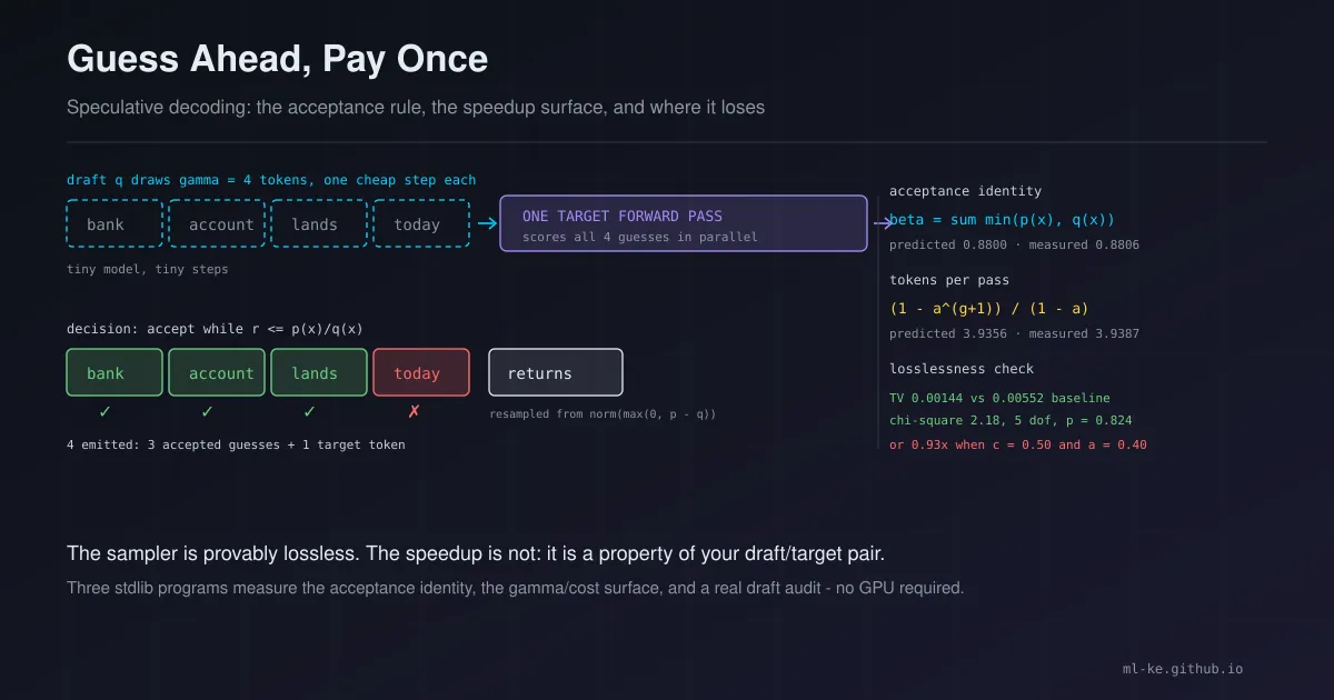
Speculative decoding is the rare inference trick that promises something for nothing: the same output distribution as the model you already run, produced with fewer sequential passes through that model. A small draft model guesses the next $\gamma$ tokens; the target model scores all of them in one forward pass; a rejection rule decides how many guesses survive. Published results are real — 2–3× on T5-XXL, 2–2.5× on Chinchilla 70B, 1.61× measured on a consumer laptop, and up to 6.5× claimed for EAGLE-3.

The part the benchmark tables hide Accepted guesses only help if verifying them is cheaper than generating them one at a time. In a recent five-configuration study on consumer hardware, three of five configurations ran slower than plain decoding, and the same EAGLE-3 method that posts a 6.5× single-stream number drops to 1.38× throughput at a batch size of 64.

This post is the measurement layer under those claims. Three short programs, no GPU and no model download: one proves the sampler is lossless, one maps the speedup surface where speculation pays, and one audits a real draft/target pair. The siblings on this blog cover adjacent levers — KV cache quantization trades bytes for accuracy in memory, constrained decoding shapes which tokens are legal at all — while this one is about the decode loop’s own latency.

The rule, in four lines

Let $p$ be the target model’s next-token distribution and $q$ the draft model’s. Draw $\gamma$ tokens from $q$, then score them with $p$ in a single batched pass. Accept token $i$ while a uniform draw satisfies $r_i \le p(x_i)/q(x_i)$; at the first rejection, sample the replacement from the residual distribution

\[p'(x) = \mathrm{norm}\big(\max(0, p(x) - q(x))\big)\]

and if every guess survives, take one extra token from $p$ — the pass was already paid for. The acceptance probability of a drafted token has a closed form (Leviathan et al., §3):

\[\beta = \sum_x \min\big(p(x), q(x)\big), \qquad \mathbb{E}[\text{tokens per target pass}] = \frac{1-\alpha^{\gamma+1}}{1-\alpha}\]

with $\alpha$ the mean acceptance rate. Those two equations are the whole economics of the technique: acceptance is a property of the pair $(p, q)$, and tokens per pass saturates as $\gamma$ grows.

Proof before performance: the sampler is lossless

“Lossless” is a strong claim, so measure it. This program runs 50,000 speculative cycles against a six-token vocabulary and compares the emitted token distribution with a plain autoregressive baseline sampling straight from $p$.

import math, random
random.seed(20261002)

VOCAB = ["the", "of", "and", "Kenya", "model", "."]
P = [0.38, 0.22, 0.16, 0.12, 0.08, 0.04]    # target model p
Q = [0.30, 0.20, 0.20, 0.10, 0.14, 0.06]    # draft  model q
GAMMA, CYCLES = 4, 50_000


def draw(dist):
    r, acc = random.random(), 0.0
    for i, w in enumerate(dist):
        acc += w
        if r <= acc:
            return i
    return len(dist) - 1


def residual(p, q):                      # p' = norm(max(0, p - q))
    d = [max(0.0, a - b) for a, b in zip(p, q)]
    s = sum(d)
    return [x / s for x in d]


def spec_cycle():                        # Leviathan et al., Algorithm 1
    draft = [draw(Q) for _ in range(GAMMA)]
    accepted = evaluated = 0
    for tok in draft:
        evaluated += 1                   # the target scored this position
        if random.random() > P[tok] / Q[tok]:
            return draft[:accepted] + [draw(residual(P, Q))], accepted, evaluated
        accepted += 1
    return draft + [draw(P)], accepted, evaluated     # all accepted -> bonus token


def upper_gamma(a, x):                   # Q(a, x), regularized upper incomplete gamma
    gln, ap, s, d = math.lgamma(a), a, 1.0 / a, 1.0 / a
    for _ in range(1000):
        ap += 1
        d *= x / ap
        s += d
        if abs(d) < abs(s) * 1e-14:
            break
    return 1.0 - s * math.exp(-x + a * math.log(x) - gln)


spec_c, direct_c = [0] * len(VOCAB), [0] * len(VOCAB)
accepted_total = evaluated_total = emitted = 0
for _ in range(CYCLES):
    toks, acc, ev = spec_cycle()
    for t in toks:
        spec_c[t] += 1
    emitted += len(toks)
    accepted_total += acc
    evaluated_total += ev
    direct_c[draw(P)] += 1               # plain autoregressive baseline: one call per token

alpha = sum(min(a, b) for a, b in zip(P, Q))
tv = lambda c: 0.5 * sum(abs(c[i] / sum(c) - P[i]) for i in range(len(P)))
n = sum(spec_c)
chi2 = sum((spec_c[i] - n * P[i]) ** 2 / (n * P[i]) for i in range(len(P)))

print(f"acceptance: theory sum min(p,q) = {alpha:.4f}   measured = {accepted_total / evaluated_total:.4f}")
print(f"tokens per target pass: theory {(1 - alpha ** (GAMMA + 1)) / (1 - alpha):.4f}   measured = {emitted / CYCLES:.4f}   (gamma = {GAMMA})")
print(f"TV distance to p: speculative {tv(spec_c):.5f}   plain AR baseline {tv(direct_c):.5f}")
print(f"chi-square (5 dof) = {chi2:.2f}   p-value = {upper_gamma(2.5, chi2 / 2):.3f}")
print(f"{emitted} tokens emitted from {CYCLES} target passes, {accepted_total} of {evaluated_total} scored positions accepted")

acceptance: theory sum min(p,q) = 0.8800   measured = 0.8806
tokens per target pass: theory 3.9356   measured = 3.9387   (gamma = 4)
TV distance to p: speculative 0.00144   plain AR baseline 0.00552
chi-square (5 dof) = 2.18   p-value = 0.824
196936 tokens emitted from 50000 target passes, 146936 of 166865 scored positions accepted

Four readings, all of them the ones to log in production:

• The acceptance identity holds. Measured acceptance is 0.8806 against a predicted $\sum_x \min(p(x), q(x)) = 0.8800$ — the identity is not an approximation you inherit, it is a quantity you can predict before you deploy.
• Tokens per pass matches the formula. 3.9387 measured against 3.9356 predicted at $\gamma = 4$: this is the number that converts acceptance into a latency budget.
• The output is statistically indistinguishable from the target. Total-variation distance to $p$ is 0.00144 for speculative sampling versus 0.00552 for the plain baseline — both are finite-sample noise around the same distribution, and the speculative run is not the worse of the two.
• A chi-square test agrees. $\chi^2 = 2.18$ at 5 degrees of freedom gives $p = 0.824$; there is no evidence the two paths differ. The $p$-value is computed with a fifteen-line incomplete-gamma routine so the check stays dependency-free.

Do not “verify” losslessness with a random seed and eyeballs. Sampling is stochastic; the only defensible checks are distributional (TV distance, chi-square) plus exact-match on greedy decoding, which is what the paper by Chordiya (2026) reports at three levels, ending in $\chi^2 = 162.5$ with dof 200 and $p = 0.976$ over roughly 9,200 real-model tokens.

The speedup surface: acceptance is only half the story

Acceptance tells you how many tokens you get; the cost of the draft tells you what you paid. With $c$ the draft step’s cost as a fraction of a target step, one speculative cycle costs $1 + \gamma c$ target-step equivalents to produce $\frac{1-\alpha^{\gamma+1}}{1-\alpha}$ tokens. That is a two-variable optimisation over $\gamma$:

def speedup(alpha, gamma, c):
    """Leviathan eq. 1 divided by the per-cycle cost (1 target call + gamma draft calls)."""
    return ((1 - alpha ** (gamma + 1)) / (1 - alpha)) / (1 + gamma * c)


print("best gamma and speedup by acceptance rate (draft costs c x a target step)")
print(f"{'alpha':>6} | {'c=0.10':>16} | {'c=0.30':>16} | {'c=0.50':>16}")
for alpha in (0.4, 0.5, 0.6, 0.7, 0.8, 0.9):
    cells = []
    for c in (0.10, 0.30, 0.50):
        best = max(((speedup(alpha, g, c), g) for g in range(1, 9)))
        cells.append(f"{best[0]:.2f}x at g={best[1]}")
    print(f"{alpha:>6.2f} | {cells[0]:>16} | {cells[1]:>16} | {cells[2]:>16}")

print()
print("where speculation LOSES (alpha = 0.40, c = 0.50):")
for g in (1, 2, 4, 6, 8):
    print(f"  gamma={g}: {speedup(0.40, g, 0.50):.3f}x")
print()
print("same draft quality, cheaper draft (alpha = 0.40, c = 0.05):")
for g in (1, 2, 4, 6, 8):
    print(f"  gamma={g}: {speedup(0.40, g, 0.05):.3f}x")

best gamma and speedup by acceptance rate (draft costs c x a target step)
 alpha |           c=0.10 |           c=0.30 |           c=0.50
  0.40 |     1.30x at g=2 |     1.08x at g=1 |     0.93x at g=1
  0.50 |     1.46x at g=2 |     1.15x at g=1 |     1.00x at g=1
  0.60 |     1.67x at g=3 |     1.23x at g=1 |     1.07x at g=1
  0.70 |     1.98x at g=4 |     1.37x at g=2 |     1.13x at g=1
  0.80 |     2.47x at g=6 |     1.55x at g=3 |     1.22x at g=2
  0.90 |     3.40x at g=8 |     1.87x at g=5 |     1.38x at g=3

where speculation LOSES (alpha = 0.40, c = 0.50):
  gamma=1: 0.933x
  gamma=2: 0.780x
  gamma=4: 0.550x
  gamma=6: 0.416x
  gamma=8: 0.333x

same draft quality, cheaper draft (alpha = 0.40, c = 0.05):
  gamma=1: 1.333x
  gamma=2: 1.418x
  gamma=4: 1.375x
  gamma=6: 1.280x
  gamma=8: 1.190x

Three things fall out of the table:

1. The optimal $\gamma$ is small and falls as drafting gets expensive. At $c = 0.30$ and $\alpha = 0.80$ the best guess length is 3; at $c = 0.50$ it is 2. Long drafts are a losing trade, which is why llama-server defaults to --spec-draft-n-max 3.
2. A mediocre draft at a bad price is a pessimisation. With $\alpha = 0.40$ and $c = 0.50$, every guess length is slower than not speculating — 0.93× at $\gamma = 1$, 0.33× at $\gamma = 8$. This is not a corner case; it is what three of five configurations measured in the consumer-hardware study: the draft failed to out-speed the target, or the “parallel” verification ran serially on the quantized backend.
3. Cost ratio, not acceptance, is the first thing to fix. Hold $\alpha = 0.40$ and drop $c$ from 0.50 to 0.05 and the same weak draft becomes a 1.42× win at $\gamma = 2$. If your draft model costs half a target step, no amount of tuning saves you; if it costs a twentieth, even a poor drafter pays.

Audit the draft you actually have

Published numbers come from someone else’s model pair. The number that matters is yours. This program trains two cheap unsupervised drafts — a unigram and a bigram model — against an interpolated trigram target on a 297-token corpus (237 tokens train, 60 held out, 131-word vocabulary), then reports both the predicted acceptance and the acceptance observed by running the actual rejection rule on held-out positions.

import random
random.seed(11)

CORPUS = """
Nairobi is the capital of Kenya and the largest city in East Africa. Mobile money moved
money in Kenya long before cards did, and today almost every shop accepts a payment on a
phone. Banks and mobile money operators now run their own rails, so a payment can leave a
bank account and land in a mobile wallet in seconds. That speed changed how small shops
manage cash, and it changed how builders write software for payments. A developer in
Nairobi now builds on the same rails a bank uses, which means the same rules apply to a
small shop and to a large lender. When a payment fails, the money must return to the
account that sent it, and the record of that failure must survive the next day. Teams
that ignore the record pay for it later, because a failed payment is a support ticket and
a reconciliation break at the same time. The teams that do well keep a clear record of
every state change, and they test the failure path as often as they test the happy path.
Kenya also builds for devices that cost less than a laptop, and that constraint shapes
the software. A model that runs on a phone must be small, and a model that runs on a
server must be cheap to serve. Serving cost matters most when traffic arrives in bursts,
because capacity bought for the peak sits idle during the quiet hours. Engineers in
Nairobi solve this the same way engineers solve it everywhere: measure first, then cut
what the measurement shows to be waste. Measure the latency, measure the cost, and keep
the record of both. A record kept by hand drifts, and a record kept by a machine can be
read again next month.
"""

SMOOTH = 0.02
toks = CORPUS.lower().split()
cut = int(len(toks) * 0.8)
train, test = toks[:cut], toks[cut:]
vocab = sorted(set(train))
V = len(vocab)


def counts(data, n):
    c = {}
    for i in range(len(data) - n + 1):
        c[tuple(data[i:i + n])] = c.get(tuple(data[i:i + n]), 0) + 1
    return c


c1, c2, c3 = counts(train, 1), counts(train, 2), counts(train, 3)
uni = {w: (c1.get((w,), 0) + SMOOTH) / (len(train) + SMOOTH * V) for w in vocab}


def cond(table, ctx, ctx_counts):        # p(w | ctx) for an n-gram table
    denom = ctx_counts.get(ctx, 0) + SMOOTH * V
    return {w: (table.get(ctx + (w,), 0) + SMOOTH) / denom for w in vocab}


def draw(dist):
    r, run = random.random(), 0.0
    for w, pr in dist.items():
        run += pr
        if r <= run:
            return w
    return w


def target(a, b):                        # interpolated trigram: the model to reproduce
    t, g = cond(c3, (a, b), c2), cond(c2, (b,), c1)
    return {w: 0.7 * t[w] + 0.2 * g[w] + 0.1 * uni[w] for w in vocab}


def unigram_draft(a, b):
    return uni


def bigram_draft(a, b):
    return cond(c2, (b,), c1)


def evaluate(q_fn, trials=10):
    beta, acc, n = 0.0, 0, 0
    for i in range(2, len(test)):
        a, b = test[i - 2], test[i - 1]
        p, q = target(a, b), q_fn(a, b)
        assert abs(sum(p.values()) - 1) < 1e-9 and abs(sum(q.values()) - 1) < 1e-9
        beta += sum(min(p[w], q[w]) for w in vocab)
        for _ in range(trials):
            x = draw(q)
            n += 1
            acc += random.random() <= min(1.0, p[x] / q[x])
    beta /= len(test) - 2
    best = max(((1 - beta ** (g + 1)) / (1 - beta) / (1 + g * 0.3), g) for g in range(1, 9))
    print(f"{q_fn.__name__:14s} beta={beta:.3f} observed_accept={acc / n:.3f} (n={n})"
          f"  -> best {best[0]:.2f}x at gamma={best[1]}")


print(f"corpus {len(toks)} tokens | vocab {V} | train {len(train)} | held out {len(test)}")
print("both distributions normalise to 1.0 on every held-out position")
evaluate(unigram_draft)
evaluate(bigram_draft)

corpus 297 tokens | vocab 131 | train 237 | held out 60
both distributions normalise to 1.0 on every held-out position
unigram_draft  beta=0.706 observed_accept=0.717 (n=580)  -> best 1.38x at gamma=2
bigram_draft   beta=0.798 observed_accept=0.791 (n=580)  -> best 1.55x at gamma=3

Read the gap between the two drafts, not the absolute numbers: a draft that knows nothing about word order accepts 0.706 of its guesses, while a draft one order higher — still trivially cheap — accepts 0.798. At a draft cost of 0.3 target steps, that is the difference between 1.38× and 1.55×, and the level of agreement between predicted beta and observed acceptance (0.011 and 0.007 apart over 580 trials) is what tells you the measurement is wired up correctly.

The assert is not padding. The first version of this script read context counts out of the wrong n-gram table, so $\sum_x \min(p, q)$ exceeded 1.0 and the predicted speedup was nonsense; a distribution that does not sum to 1 on every position is the fastest way to catch that class of bug. Also note the honest limit of a toy pair: real vocabularies hold 100k+ tokens and real target distributions are far sharper than a smoothed trigram, which is why same-family drafts land near 0.7 acceptance at $K=1$ and decay to about 0.38 by the optimum in Chordiya’s measurements — well below this corpus’s 0.71–0.80.

Where it backfires at scale

The single-stream story is the one that gets quoted. The serving story is where teams get burned.

Regime	What changes	Reported outcome	Source
Single stream, matched draft	Verification is genuinely batch-parallel and the draft is much cheaper	1.61× wall-clock at $K=6$; three of five configurations decelerate instead	Chordiya 2026, arXiv:2607.17283
High concurrency	Drafting competes with the real workload for compute; batches desynchronise	EAGLE-3’s 6.5× single-stream speedup becomes 1.38× throughput at batch 64 in SGLang	Li et al. 2025, arXiv:2503.01840
Batched serving correctness	Variable acceptance desynchronises position IDs, masks, and KV cache	Several widely used implementations silently emit repetitive tokens while reporting competitive speed; fixes reach 3× at batch 8 with 95% exact match	Zhang et al. 2026, arXiv:2510.22876
Production serving with batching	Speculation must not destroy throughput at larger batch sizes	Required a modified paged-attention kernel; deployed at 2× (8B/13B/7B models) and 3× (20B code model)	PyTorch/IBM, Hitchhiker’s Guide
Framework scope	vLLM documents the feature for medium-to-low QPS, memory-bound latencies; pipeline parallelism is not composable with it	Method-dependent gains, no draft model needed for n-gram and suffix variants	vLLM docs

Two operational cautions that follow from that table:

• Lossless is not bitwise identical. vLLM’s own documentation notes that token log probabilities are not guaranteed stable across runs and that batch-size changes alter outputs through floating-point and numerical effects — the distribution is preserved, the byte stream is not.
• Benchmark knobs are not serving knobs. Both vLLM (rejection_sample_method: synthetic, synthetic_acceptance_rates) and llama.cpp (--spec-synth-rates, --spec-synth-len) can replace real verification with synthetic acceptance probabilities to isolate a bottleneck. llama.cpp’s docs are blunt that the resulting output “is not valid model output”. Use them to size a hypothesis, never to demo quality.

How to apply this

1. Predict $\beta$ before you spend a GPU-hour. For any position you can log, $\sum_x \min(p(x), q(x))$ is a one-pass computation over two distribution vectors. If the predicted acceptance is under about 0.5 with a draft that costs more than a fifth of a target step, stop and fix the pair.
2. Measure the cost ratio, not the model sizes. What matters is your measured draft-step to target-step latency on your hardware. The same pair scores 0.93× or 1.42× depending only on that ratio in the table above.
3. Sweep $\gamma$ on the acceptance you actually measured. Use the grid above: the optimum is 2–5 in most healthy configurations, and it moves toward 1 as drafting gets expensive.
4. Log acceptance per position, not just the mean. Early positions are accepted far more often than late ones; a falling profile is the early signal that your draft is drifting off the target’s distribution. vLLM exposes per-request acceptance metrics for exactly this.
5. Prove the output path. Run a greedy decode with and without speculation and diff the token sequences; then run the distributional check from the first program. If either fails, the “speedup” is a different model answering.
6. Only then scale the batch. Re-measure the throughput curve at your production concurrency, because the single-stream result does not transfer.

Framework configurations, both verified from the projects’ own docs:

# vLLM: model-based drafting, then a cheap no-model variant to compare against
vllm serve Qwen/Qwen3-4B \
  --speculative-config '{"method": "draft_model", "model": "<draft-model>", "num_speculative_tokens": 5}'

vllm serve Qwen/Qwen3-4B \
  --speculative-config '{"method": "ngram", "num_speculative_tokens": 4, "prompt_lookup_min": 2, "prompt_lookup_max": 5}'

# llama.cpp: draft model (default 3 draft tokens), then the no-draft n-gram path
llama-server -m target.gguf -md draft.gguf --spec-type draft-simple --spec-draft-n-max 3
llama-server -m target.gguf --spec-type ngram-mod

The no-draft variants matter for teams with one model in the box: n-gram and suffix drafting copy continuations the context has already seen, so they cost no extra weights and pay off best where the output echoes the context — iterating over a block of text or code, summarisation, and reasoning models that restate their thinking, which are the cases llama.cpp documents for its ngram-mod mode.

A draft is not just a smaller model

Pairing rules matter more than draft size. The measured examples in the wild are almost all same-family pairs — Qwen2.5-32B with a Qwen2.5-0.5B draft, Llama-3.1-8B with a Llama-3.2-1B draft — and the payoff moves with how predictable the output is. On LM Studio’s own benchmarks, the same 8B/1B Llama pair goes from 29.65 to 50.91 tokens/sec (1.71×) on conversational prompts and hits 2.43× with a 32B Qwen target on a code-only prompt, where the continuation is highly constrained. Their release notes also carry the warning that belongs next to every speedup chart: “In cases where tokens are rejected more often than not, you will likely see decreased total generation speed!”

If no same-family draft exists, vLLM’s use_heterogeneous_vocab: true enables a token-level intersection so drafts from a different family can be used at all, with the draft’s logits constrained to the shared tokens — a workable fallback, not a free lunch, since the intersection discards the draft’s vocabulary advantage. The alternative that avoids the question entirely is training a speculator or multi-token-prediction head against the exact target, which is what EAGLE-3, MTP-based drafts and vLLM’s speculators project do, and why their acceptance profiles hold up as training data scales.

Key takeaways

Finding	Number	What to do with it
Acceptance equals $\sum_x \min(p, q)$	0.8806 measured vs 0.8800 predicted	Predict $\beta$ from logged distributions before deploying
Tokens per target pass follow the capped-geometric formula	3.9387 measured vs 3.9356 predicted at $\gamma=4$	Convert acceptance into a latency budget, don’t guess
The sampler is lossless, measurably	TV 0.00144 vs 0.00552 baseline; $\chi^2$ p = 0.824	Verify with a distributional test plus greedy exact-match
The optimum guess length is small	Best $\gamma$ of 2–5 for healthy pairs; 3 is llama.cpp’s default	Sweep $\gamma$ against your measured cost ratio
Speculation can lose	0.93× at $\alpha=0.40$, $c=0.50$	Fix the cost ratio before tuning anything else
Draft quality is worth a lot	$\beta$ 0.706 → 0.798 from unigram to bigram on the same corpus	Spend on draft/target alignment (EAGLE-3, MTP, same-family draft)
Concurrency rewrites the answer	6.5× single stream → 1.38× throughput at batch 64	Re-measure at production batch size, and check correctness at batch

References

• Leviathan, Kalman & Matias (2023). Fast Inference from Transformers via Speculative Decoding. ICML 2023 Oral. arXiv:2211.17192 — Algorithm 1, the acceptance identity, and the expected-tokens formula.
• Chen et al. (2023). Accelerating Large Language Model Decoding with Speculative Sampling. arXiv:2302.01318 — 2–2.5× on Chinchilla 70B; the modified rejection-sampling scheme.
• Chordiya, P. (2026). Lossless but Not Free: An Empirical Anatomy of Speculative Decoding on Consumer Hardware. arXiv:2607.17283 — 1.61× at $K=6$, acceptance 69.7% → 37.8%, three of five configurations decelerate, $\chi^2 = 162.5$, dof 200, $p = 0.976$ over ~9,200 tokens.
• Zhang et al. (2026). Correctness Forensics for Batch Speculative Decoding: Diagnosing the Ragged Tensor Problem. Findings of EMNLP 2026. arXiv:2510.22876 — silent output corruption under batching; EXSPEC at 3× throughput, batch 8, 95% exact match.
• Li et al. (2025). EAGLE-3: Scaling up Inference Acceleration of Large Language Models via Training-Time Test. arXiv:2503.01840 — up to 6.5× speedup; 1.38× throughput at batch size 64 in SGLang.
• Team PyTorch & IBM (2024). A Hitchhiker’s Guide to Speculative Decoding. pytorch.org — paged-attention changes for batched verification; 2× and 3× in an internal production deployment.
• vLLM docs. Speculative Decoding. docs.vllm.ai — method selection table, --speculative-config schema, n-gram and suffix keys, lossless-guarantee tests, pipeline-parallel incompatibility.
• llama.cpp docs. speculative.md. github.com/ggml-org/llama.cpp — --spec-type, --spec-draft-model, --spec-draft-n-max default of 3, synthetic-acceptance flags.
• LM Studio (2025). LM Studio 0.3.10: Speculative Decoding. lmstudio.ai — same-family benchmark tables (29.65 → 50.91 tok/sec; 2.43× on a code-only prompt) and the warning that frequent rejections reduce generation speed.

Related posts

• KV Cache Quantization at Long Context: the Bytes Halve, the Accumulator Does Not
• The Mask Is the Contract: Grammar-Constrained Decoding
• vLLM and the Anatomy of LLM Serving
• Self-Hosting Open-Weight LLMs
• Auditing Embedding Compression Before You Ship It
• MinHash + LSH: Your Corpus Is Duplicating Itself