How Many Lists, How Many Probes: Sizing an IVF Index Against a Recall Budget

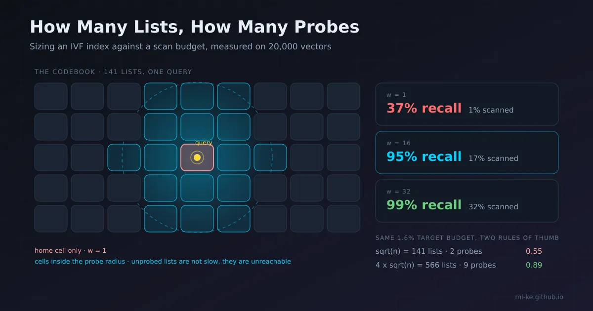
The short version An inverted-file index splits the corpus into nlist cells and answers a query by scanning only the nprobe cells closest to it. Every guide names the same two dials and then suggests a different starting value for them. The number that actually governs recall is neither: it is the fraction of the corpus you allow a query to touch. State that fraction first and both rules of thumb become checkable.

Two documents, two defaults

The advice floating around production teams is not wrong, it is just stated at different scales.

Source	Lists	Probes
ZeroEntropy concept page	about sqrt(N): 1024 lists at 1M vectors, 16384 at 100M	8 to 64 for 95%+ recall
Milvus performance FAQ	4 × sqrt(n), where n is entities per segment	set by experiment
Faiss index factory	IVF4096 means 4096 centroids over a flat quantiser	set at search time

The gap between the first two rows is a factor of four in lists. At a fixed scan budget that becomes a factor of four in probes, which is a difference you can measure rather than argue about. Milvus also attaches its rule to a segment rather than a collection, and a segment defaults to 512 MB, so the n in its formula is whatever fits in that box, not the total corpus size.

Worth naming what IVF is for, because the choice of index decides whether any of this matters. A cell partition stores one id per vector and nothing else, so its per-vector overhead is small: 8 bytes per entry on top of the embedding itself, per the Faiss documentation. A graph index spends far more on links. The same documentation puts HNSW32 at 256 bytes per vector, which on a million vectors is 244 MiB of graph against 7.6 MiB of ids, a factor of 32. IVF is the index you pick when memory binds, and the price of that choice is the cell-boundary recall loss measured below. If memory is not the constraint, a graph index may simply be better and this article is not the one you need.

The cost formula you cannot skip

Jégou, Douze and Schmid wrote down the accounting for this structure in the product-quantisation paper that introduced the inverted-file variant of it. Two sentences carry the whole sizing argument:

Assuming that the inverted lists are balanced, about n × w/k₀ entries have to be parsed.

The proportion of the dataset to visit is roughly linear in w/k₀.

Here w is the number of cells probed and k₀ the number of cells. The consequence is immediate: a scan budget is a ratio, not a count. Ask for 1% of a million rows and you have 10,000 rows to score per query, and any (k₀, w) pair with w/k₀ = 0.01 fits that bill. The same paper reports the finding that decides between the two vendor rules: hold the proportion fixed and raise k₀, and recall improves. Their example compares (k₀ = 1024, w = 1) against (k₀ = 8192, w = 8), both at one part in 1024 of the corpus.

There is a second cost the ratio hides. Every query computes k₀ distances against the centroids before it touches a single vector, so a larger cell count is not free at a fixed budget. That tax is worth arithmetic later; first, the recall side.

Build one and sweep the probe count

The demo below builds an IVF index from scratch in numpy, using synthetic embeddings drawn from 200 clusters because real embeddings clump and uniform noise does not. Centroids are trained on an 8,000-vector sample rather than the whole corpus, which keeps the training cost bounded at the price of a slightly noisier partition. Recall is measured against an exact brute-force top-10.

import numpy as np

RNG = np.random.default_rng(7)
N, D, K, k0 = 20000, 32, 10, 141

def corpus(n, d=D, blobs=200, spread=0.45):
    centers = RNG.normal(0, 1, (blobs, d))
    return centers[RNG.choice(blobs, size=n)] + RNG.normal(0, spread, (n, d))

def sqdist(A, B):                      # |a|^2 + |b|^2 - 2ab, no (n, m, d) tensor
    return (A * A).sum(1)[:, None] + (B * B).sum(1)[None, :] - 2.0 * A @ B.T

def kmeans(X, k, iters=12):
    C = X[RNG.choice(len(X), k, replace=False)].copy()
    for _ in range(iters):
        a = sqdist(X, C).argmin(1)
        for j in range(k):
            if (a == j).any():
                C[j] = X[a == j].mean(0)
    return C

X, Q = corpus(N), corpus(500)
C = kmeans(X[RNG.choice(N, 8000, replace=False)], k0)   # train on a sample
cell = sqdist(X, C).argmin(1)
lists = [np.flatnonzero(cell == j) for j in range(k0)]
order = sqdist(Q, C).argsort(1)                          # cells, nearest first
truth = sqdist(Q, X).argsort(1)[:, :K]

sizes = np.array([len(l) for l in lists])
print(f"lists mean={sizes.mean():.1f} max={sizes.max()} min={sizes.min()}")
print("nprobe | corpus scanned | recall@10")
hit = {}
for w in (1, 2, 4, 8, 16, 32, 64, k0):
    found, scanned = [], 0
    for i, row in enumerate(order):
        cand = np.concatenate([lists[j] for j in row[:w]])
        scanned += len(cand)
        found.append(cand[np.argsort(sqdist(Q[i:i+1], X[cand])[0])[:K]])
    hit[w] = np.mean([len(set(a) & set(b)) / K for a, b in zip(found, truth)])
    print(f"{w:6d} | {scanned/(len(Q)*N)*100:13.2f}% | {hit[w]:.3f}")

print("first nprobe at or above 0.95 recall:",
      min(w for w, r in hit.items() if r >= 0.95))

Run it with uv run --with=numpy python3 ivf.py (or any interpreter with numpy installed). The output:

lists mean=141.8 max=344 min=2
nprobe | corpus scanned | recall@10
     1 |          1.09% | 0.372
     2 |          2.18% | 0.549
     4 |          4.38% | 0.740
     8 |          8.65% | 0.859
    16 |         16.80% | 0.948
    32 |         32.01% | 0.991
    64 |         58.14% | 1.000
   141 |        100.00% | 1.000
first nprobe at or above 0.95 recall: 32

Three things in that table matter more than the recall numbers themselves.

The first probe is a lottery ticket. With w = 1 you score 1.09% of the corpus and recover 37% of the true neighbours, so nearly two thirds of your ranking is wrong before scoring even starts, and no reranker downstream can fix what pruning discarded.

Recall climbs fastest over the first two doublings, gaining 17.7 and then 19.1 points, and flattens after that: 11.9 points from 4 probes to 8, 8.9 from 8 to 16, then 4.3 from 16 to 32. That bend is the useful part of the curve. Below it each doubling of the probe count buys real recall; above it the next 15 points of corpus scanned buy 4.3 points of recall.

The crossing point is specific. On this corpus 95% recall lands at 32 probes, not at 16, and the folklore figure of “16 probes for 95%” (which the ZeroEntropy page and several vendor blogs repeat) came in at 94.8% here. That is not a contradiction, it is a reminder that the crossing sits wherever your corpus puts it, and 0.2 points is enough to fail a service-level target.

One structural note from the first line: the largest list holds 344 vectors while the smallest holds 2, a spread of 172× despite a mean of 141.8.

Hold the budget fixed, then move the cell count

The comparison the two vendor rules imply needs a controlled test: same scan budget, different nlist, nprobe chosen to match. That is the block below. Note the target column, not the achieved one: w has to be an integer, and unbalanced lists mean the achieved fraction drifts a few tenths off target.

import numpy as np

RNG = np.random.default_rng(7)
N, D, K = 20000, 32, 10

def corpus(n, d=D, blobs=200, spread=0.45):
    centers = RNG.normal(0, 1, (blobs, d))
    return centers[RNG.choice(blobs, size=n)] + RNG.normal(0, spread, (n, d))

def sqdist(A, B):
    return (A * A).sum(1)[:, None] + (B * B).sum(1)[None, :] - 2.0 * A @ B.T

def kmeans(X, k, iters=12):
    C = X[RNG.choice(len(X), k, replace=False)].copy()
    for _ in range(iters):
        a = sqdist(X, C).argmin(1)
        for j in range(k):
            if (a == j).any():
                C[j] = X[a == j].mean(0)
    return C

X, Q = corpus(N), corpus(500)
truth = sqdist(Q, X).argsort(1)[:, :K]

print("scan target | k0  | nprobe | actual scan | recall@10 | centroid dists/query")
for target in (1/64, 1/32, 1/16):
    for k0 in (141, 283, 566, 1024):
        w = max(1, round(target * k0))
        C = kmeans(X[RNG.choice(N, 8000, replace=False)], k0)
        cell = sqdist(X, C).argmin(1)
        lists = [np.flatnonzero(cell == j) for j in range(k0)]
        order = sqdist(Q, C).argsort(1)
        found, scanned = [], 0
        for i, row in enumerate(order):
            cand = np.concatenate([lists[j] for j in row[:w]])
            scanned += len(cand)
            found.append(cand[np.argsort(sqdist(Q[i:i+1], X[cand])[0])[:K]])
        rec = np.mean([len(set(a) & set(b)) / K for a, b in zip(found, truth)])
        print(f"{target:11.4f} | {k0:4d} | {w:6d} | {scanned/(len(Q)*N)*100:10.2f}% | {rec:.4f}    | {k0:5d}")

scan target | k0  | nprobe | actual scan | recall@10 | centroid dists/query
     0.0156 |  141 |      2 |       2.18% | 0.5492    |   141
     0.0156 |  283 |      4 |       1.70% | 0.8206    |   283
     0.0156 |  566 |      9 |       1.77% | 0.8856    |   566
     0.0156 | 1024 |     16 |       1.78% | 0.8964    |  1024
     0.0312 |  141 |      4 |       4.44% | 0.7224    |   141
     0.0312 |  283 |      9 |       3.82% | 0.9226    |   283
     0.0312 |  566 |     18 |       3.53% | 0.9622    |   566
     0.0312 | 1024 |     32 |       3.45% | 0.9646    |  1024
     0.0625 |  141 |      9 |       9.62% | 0.9038    |   141
     0.0625 |  283 |     18 |       8.05% | 0.9906    |   283
     0.0625 |  566 |     35 |       7.00% | 0.9918    |   566
     0.0625 | 1024 |     64 |       6.89% | 0.9928    |  1024

Read the first block of four rows. At a budget of roughly 1.6%, the square-root rule gives 0.549 and the four-times-square-root rule gives 0.886. Same scan volume, 34 points of recall apart. The sqrt rule is not a tuning recommendation at this budget, it is an under-provisioned index.

Past four times, the gains flatten hard. Going from 566 lists to 1024 lists buys 1.1 points at the 1.6% budget and 0.1 points at 6.25%, while the centroid work per query nearly doubles (566 to 1024 distances). That is the trade the Jégou finding describes, and it lands on a defensible stopping rule: 4 × sqrt(n) is a good default, and beyond it you should be able to name what you are buying.

The third budget block also shows why more lists is not automatically better. At 9.62% of a 141-list index, recall is 0.904; at 7.00% of a 566-list index it is 0.992. Fewer probes, more cells, less work, better answer. What changed is the ratio.

Rows per cell is the same number twice

Convert both rules into rows per cell and the disagreement becomes concrete. At a million vectors the square-root rule gives 1,000 lists holding 1,000 rows each; the four-times rule gives 4,000 lists of 250 rows. A 1% budget is 10,000 rows per query either way, so the first index spends it in 10 probes and the second in 40.

Both then perform the same number of vector distance computations and differ only in their two overheads. The four-times index pays 4,000 centroid comparisons per query instead of 1,000, and in exchange it chooses which rows to score from a finer partition of the space. The measurement above says that trade keeps paying until roughly four times, then stops. It also depends on the partition being real: the block-1 index has a largest list at 2.4 times the mean and 172 times the smallest, so a finer partition helps only where k-means managed to split the data, which is the point of the next section.

What the corpus decides

None of the above transfers to a corpus whose structure fights the partition. Three corpora, same index parameters, same queries:

import numpy as np

RNG = np.random.default_rng(11)
N, D, K, k0 = 20000, 32, 10, 141

def corpus(kind, n=N, d=D, blobs=200, spread=0.45):
    if kind == "uniform":
        return RNG.normal(0, 1, (n, d))
    centers = RNG.normal(0, 1, (blobs, d))
    if kind == "skewed":                # one blob holds about 40 percent of rows
        w = np.ones(blobs); w[0] = blobs * 2 / 3
        pick = RNG.choice(blobs, size=n, p=w / w.sum())
    else:
        pick = RNG.choice(blobs, size=n)
    return centers[pick] + RNG.normal(0, spread, (n, d))

def sqdist(A, B):
    return (A * A).sum(1)[:, None] + (B * B).sum(1)[None, :] - 2.0 * A @ B.T

def kmeans(X, k, iters=12):
    C = X[RNG.choice(len(X), k, replace=False)].copy()
    for _ in range(iters):
        a = sqdist(X, C).argmin(1)
        for j in range(k):
            if (a == j).any():
                C[j] = X[a == j].mean(0)
    return C

Q = corpus("blobs", 500)
print("corpus  | biggest cell | top1 miss | recall@1 | recall@8 | recall@16 | scan@16 p50/p95/max")
for kind in ("uniform", "blobs", "skewed"):
    X = corpus(kind)
    truth = sqdist(Q, X).argsort(1)[:, :K]
    C = kmeans(X[RNG.choice(N, 8000, replace=False)], k0)
    cell = sqdist(X, C).argmin(1)
    lists = [np.flatnonzero(cell == j) for j in range(k0)]
    sizes = np.array([len(l) for l in lists])
    order = sqdist(Q, C).argsort(1)
    miss = np.mean([cell[n] != order[i][0] for i, n in enumerate(truth[:, 0])])
    cells = []
    for w in (1, 8, 16):
        found, scans = [], []
        for i, row in enumerate(order):
            cand = np.concatenate([lists[j] for j in row[:w]])
            scans.append(len(cand))
            found.append(cand[np.argsort(sqdist(Q[i:i+1], X[cand])[0])[:K]])
        rec = np.mean([len(set(a) & set(b)) / K for a, b in zip(found, truth)])
        cells.append((rec, np.array(scans) / N))
    p = lambda a, q: int(round(np.quantile(a, q) * 100))
    print(f"{kind:7s} | {sizes.max()/N*100:11.2f}% | {miss:9.3f} | {cells[0][0]:.3f}    | "
          f"{cells[1][0]:.3f}    | {cells[2][0]:.3f}     | "
          f"{p(cells[2][1], .5)}%/{p(cells[2][1], .95)}%/{p(cells[2][1], 1.0)}%")

corpus  | biggest cell | top1 miss | recall@1 | recall@8 | recall@16 | scan@16 p50/p95/max
uniform |        1.00% |     0.826 | 0.128    | 0.473    | 0.657     | 12%/12%/13%
blobs   |        2.17% |     0.576 | 0.393    | 0.885    | 0.962     | 17%/20%/22%
skewed  |        2.21% |     0.614 | 0.349    | 0.831    | 0.937     | 18%/20%/21%

The uniform row is the caution. A corpus with no cluster structure is partitioned into cells that are all equally plausible neighbours, so 82.6% of queries have their true nearest neighbour in a cell that is not the nearest cell. Scanning 12% of a perfectly balanced 141-list index still recovers only 65.7% of the answer, and the missing third comes back only as the probe count approaches the whole index. If your recall target is 95%, an index over undifferentiated vectors cannot reach it at any budget short of exhaustive search. Real embeddings, which clump, land at 96.2% for the same 17%.

The skewed row is more reassuring than the vendor warnings imply. One cluster holding 40% of the corpus did not produce a giant cell, because k-means splits a dense region across several centroids; the biggest cell is 2.21% of rows, essentially the same as the balanced case, and recall falls 2.5 points. Imbalance that survives training is the kind k-means cannot separate, such as a single document indexed thousands of times. Deduplicate before indexing and this failure mode mostly disappears; skip that step and the largest cell, not the mean, sets your tail latency.

The last column is the operational figure. On the skewed corpus the median query at 16 probes scans 18% of the corpus and the worst scans 21%, a 1.2× spread on this data. On a corpus with heavy duplicates or a dense head that spread widens, and the p99 query is the one your latency budget has to cover.

Where the shortlist goes next

Pruning decides what the rest of the pipeline is allowed to see, and the handoff is a fixed-size candidate list. If you compress the vectors to score them cheaply, the scan returns candidates ranked by approximate distance and a rescore stage re-ranks the top few hundred at full precision. Two consequences follow.

The candidate list has to be wider than k, because compression loses ordering inside it, and the width of that shortlist is what buys back the recall the compression spends. And the pruning gate comes first regardless of what happens afterwards. Jégou puts the limit plainly:

Increasing the code length is useless if w is not big enough, as the nearest neighbors which are not assigned to one of the w centroids associated with the query are definitely lost.

A perfect quantiser cannot return a document whose cell was never probed. Audit the scan before you audit the compression, and treat retrieval recall as a product of the two gates rather than a property of either. The embedding compression audit works the second gate.

What recall does not capture

Recall@10 against exact top-k measures the pruning and nothing else. Three failure modes sit outside it.

Centroid drift after ingest is the practical one. New vectors join whichever cell is nearest without retraining the quantiser, so a region that grows after build time ends up represented by centroids fitted to a smaller version of itself. Recall measured at build time describes the corpus at build time, and re-clustering belongs on a schedule rather than in a postmortem.

Filters change the effective corpus per query. A tenant predicate that keeps 1% of rows means the cells you probe may hold almost nothing that passes, and the pool sizing problem is a different calculation. The filtered search post covers that case.

And k is a choice that has to match the next stage. A reranker that consumes 50 candidates is not served by a recall target stated at 10, so declare the k the downstream component actually uses and measure at that k.

Capacity arithmetic before you commit

Recall is one side of the choice; memory and per-query arithmetic are the other. Nothing here needs numpy.

n, d = 1_000_000, 384
MiB = 2 ** 20

print(f"corpus {n:,} x {d} dims, float32: raw vectors {n*d*4/MiB:,.0f} MiB")
for k0 in (1_000, 4_000):
    centroids = k0 * d * 4 / MiB
    ids = n * 8 / MiB                       # 64-bit id per entry, per the Faiss docs
    print(f"k0={k0:5,}: centroids {centroids:6.1f} MiB, ids {ids:6.1f} MiB, "
          f"scan budget 1% = {n//100:,} entries, centroid distance computations/query {k0:,}")

print("\nshare of the query's arithmetic spent on centroids (k0 / (k0 + rho*n))")
for rho in (0.005, 0.01, 0.02, 0.05):
    for k0 in (1_000, 4_000):
        share = k0 / (k0 + rho * n)
        print(f"rho={rho*100:4.1f}%  k0={k0:5,}  scanned={int(rho*n):7,}  centroid share={share*100:5.1f}%")

print("\nrule of thumb at two corpus sizes")
for n2 in (1_000_000, 100_000_000):
    a, b = int(n2 ** 0.5), int(4 * n2 ** 0.5)
    print(f"n={n2:>12,}: sqrt(n)={a:6,} -> {n2/a:8.0f} rows/cell | "
          f"4*sqrt(n)={b:6,} -> {n2/b:8.0f} rows/cell | 1% probe budget={int(0.01*n2):>10,} rows")

corpus 1,000,000 x 384 dims, float32: raw vectors 1,465 MiB
k0=1,000: centroids    1.5 MiB, ids    7.6 MiB, scan budget 1% = 10,000 entries, centroid distance computations/query 1,000
k0=4,000: centroids    5.9 MiB, ids    7.6 MiB, scan budget 1% = 10,000 entries, centroid distance computations/query 4,000

share of the query's arithmetic spent on centroids (k0 / (k0 + rho*n))
rho= 0.5%  k0=1,000  scanned=  5,000  centroid share= 16.7%
rho= 0.5%  k0=4,000  scanned=  5,000  centroid share= 44.4%
rho= 1.0%  k0=1,000  scanned= 10,000  centroid share=  9.1%
rho= 1.0%  k0=4,000  scanned= 10,000  centroid share= 28.6%
rho= 2.0%  k0=1,000  scanned= 20,000  centroid share=  4.8%
rho= 2.0%  k0=4,000  scanned= 20,000  centroid share= 16.7%
rho= 5.0%  k0=1,000  scanned= 50,000  centroid share=  2.0%
rho= 5.0%  k0=4,000  scanned= 50,000  centroid share=  7.4%

rule of thumb at two corpus sizes
n=   1,000,000: sqrt(n)= 1,000 ->     1000 rows/cell | 4*sqrt(n)= 4,000 ->      250 rows/cell | 1% probe budget=    10,000 rows
n= 100,000,000: sqrt(n)=10,000 ->    10000 rows/cell | 4*sqrt(n)=40,000 ->     2500 rows/cell | 1% probe budget= 1,000,000 rows

The centroid arrays are cheap; four thousand 384-dimension centroids cost 5.9 MiB against 1,465 MiB of raw vectors. The expensive part is the arithmetic, and it is the part people forget. At a 1% budget on a million rows, a 1,000-list index spends 9.1% of its distance computations on centroids, and a 4,000-list index spends 28.6%. Tighten the budget to 0.5% and the four-times rule spends nearly half its work locating cells. That is the honest shape of the trade: the rule that buys recall at a fixed budget buys it by spending more on the quantiser, and at very tight budgets the quantiser becomes the dominant cost.

Sizing your own index

1. Measure on your own queries. Take 200 to 500 real queries, run exact top-k, and compute recall@k for each candidate nprobe. The crossing point moves with dimensionality, cluster structure and k, and it is the only number that answers the question.
2. Choose the budget, not the probe count. Entries scanned is nprobe × average list size, which is ρ × n. Pick ρ from the latency you can afford, then find the nprobe that hits it.
3. Start at 4 × sqrt(n) for the list count, and justify anything past it. The 1× rule costs recall at tight budgets on clustered data, and 8× buys a point or two for double the quantiser work.
4. Watch the biggest cell, not the mean. Tail latency is set by the largest list a query can land in. If one list holds a percent or two of the corpus more than its peers, look for near-duplicate documents before raising nprobe.
5. Re-check after bulk ingest. New vectors join existing cells without retraining, so centroids drift away from the distribution. Recall measured at build time is a statement about the corpus at build time.
6. Report recall with the budget attached. “0.95 recall@10 at 3.5% scanned” is a specification; “0.95 recall@10” is a claim that will not survive a change of budget.

Key takeaways

Question	Answer from the measurements
Which rule, sqrt(n) or 4 × sqrt(n)?	Four times, at tight budgets: 0.886 against 0.549 at a 1.6% scan
What does recall track?	The ratio nprobe / nlist, not either value alone
Where does the curve bend?	Around 32 probes here: 99.1% recall for 32% scanned
Does a bigger cell count always help?	No. Past 4×, 1.1 points of recall for 1.8× the centroid work
What limits recall besides budget?	Corpus structure: 65.7% ceiling on uniform noise at 17% scanned
What costs money at tight budgets?	The quantiser: 28.6% of distance work at k0 = 4000, ρ = 1%
What sets tail latency?	The largest list, and the p95 query’s scan count

References

• Jégou, Douze and Schmid, Product Quantization for Nearest Neighbor Search, IEEE TPAMI 2011 — the n × w/k₀ accounting, the linear-in-w/k₀ proportion, and the (1024, 1) versus (8192, 8) comparison.
• Milvus, Performance FAQ — the 4 × sqrt(n) rule per segment, the recommendation to find nprobe by experiment, and the sift50m recall charts.
• Faiss, The index factory — IVF4096 as 4096 centroids over a flat quantiser, and the 8-byte id overhead per entry.
• ZeroEntropy, IVF clustering — the sqrt(N) starting values, the 8-to-64 probe range, and the skew and re-clustering caveats.
• Zilliz, Tuning nlist and nprobe for a target recall — nprobe as the dial that sets how many clusters a query searches, and the accuracy against speed trade.

Related posts

• Your WHERE Clause Ate the Recall — the same index under a metadata filter, where the pool has to be sized against selectivity.
• Fuse Ranks, Not Scores — what to do with the candidate list once pruning has produced it.
• Thirty Times Smaller — compressing the vectors that survive the scan, and auditing what that costs in recall.
• The Denominator Is the Metric — measuring retrieval quality when some results have no judgements at all.