Rank Is a Budget: What LoRA at r=8 Costs and Buys on an 8B Model
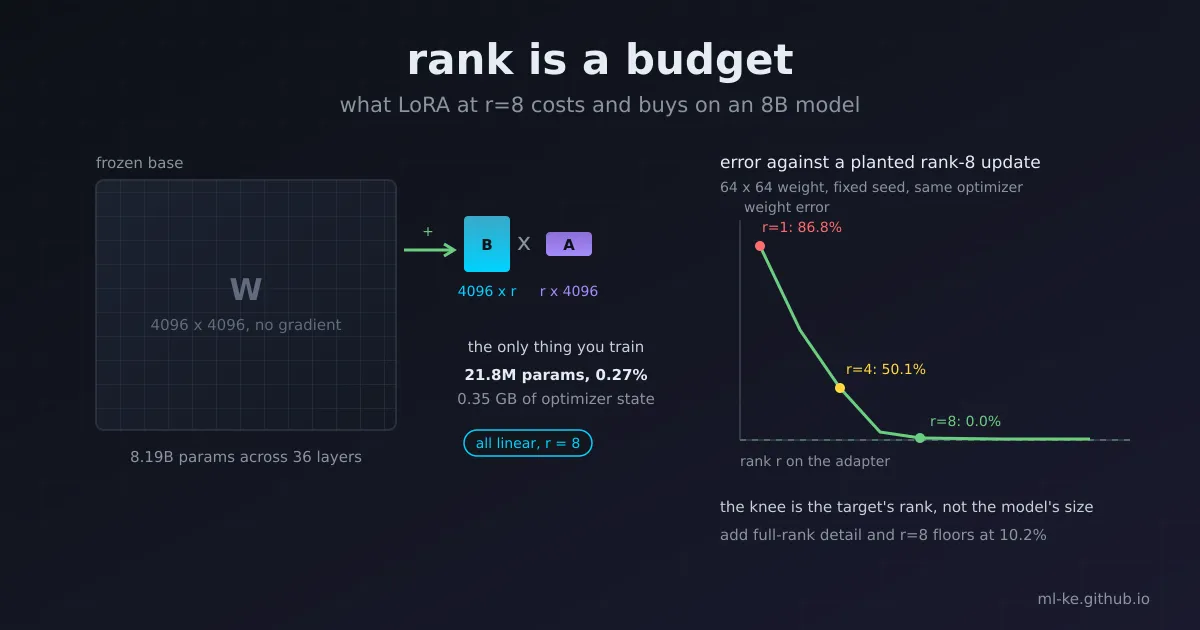
The short version LoRA spends two currencies: rank, and how many weight matrices you attach it to. On the published Qwen3-8B config, rank 8 over query and value alone trains 3.83M parameters, 0.05% of the model, for 0.06 GB of optimizer state. The same rank over all seven linear maps trains 21.8M, 0.27%, for 0.35 GB. Meanwhile the published guidance disagrees about rank itself: the original LoRA paper finds r=1 competitive on WikiSQL and MultiNLI, QLoRA finds rank irrelevant once every layer is adapted, and a 2024 study of code and math finds full fine-tuning learns perturbations 10 to 100 times higher rank than typical adapters. A planted-rank experiment resolves the tension: error collapses exactly when r reaches the target’s rank, and stays on a floor when the target carries detail outside the adapter’s subspace.
Fine-tuning advice for LoRA usually arrives as a number. Set r to 8, or 16, or 64. Use alpha equal to r, or twice r. Attach it to q and v, or to everything. Each of those numbers is defensible, and together they look like folklore because the thing being budgeted is never written down. The adapter you train is a product of two thin matrices, and its rank is a hard ceiling on the update it can represent. Everything else is a question about whether the update your task needs fits under that ceiling.
This post does the arithmetic on a real architecture, then runs two experiments small enough to finish on a laptop. The first shows where the error curve bends. The second shows what a rank cap cannot reach.
Published guidance disagrees, usefully
Four sources, one table. None of them is wrong.
| Source | Setting | Rank finding |
|---|---|---|
| Hu et al., LoRA, Table 6 | GPT-3 175B, WikiSQL and MultiNLI | r=1 matches r=64 when adapting Wq and Wv: 73.4% against 73.5% on WikiSQL, 91.3% against 91.4% on MultiNLI |
| Dettmers et al., QLoRA, appendix A.1 | LLaMA 7B to 65B, rank swept 8 to 256 | “LoRA r is unrelated to final performance if LoRA is used on all layers” |
| Biderman et al., 2024 | Code and math, both instruction tuning and continued pretraining | Full fine-tuning learns a perturbation of rank 10 to 100 times higher than typical LoRA configs; ranks 16 to 64 tend not to suffice for code |
| Park, 2026 | Binary GLUE-style tasks under cross-entropy | The sufficient-condition threshold on r collapses to 1 for binary classification, and shifts above 1 for multi-class MNLI |
Table 6 from the LoRA paper gets quoted most, usually as a single line. Read the whole thing and the claim narrows. A rank as small as one suffices for adapting Wq and Wv, but training Wq alone needs a larger r, and the paper’s own GPT-2 experiments peak at r=16 for validation loss and r=4 for BLEU. What the table shows is that the update has a small intrinsic rank for those tasks, not that rank never matters.
QLoRA’s appendix reaches the opposite conclusion about rank and then explains it away: what mattered was how many adapters were used in total. Applying LoRA to every linear transformer block layer was what matched 16-bit full fine-tuning, and once that was fixed, the projection dimension stopped moving the result. Rank, in that setting, was slack.
Biderman and colleagues measured why the slack runs out. On code and math, the perturbation full fine-tuning learns keeps growing in rank as training proceeds, well above what an r=8 or r=16 adapter can represent, which is why they recommend rank 256 on all modules when memory allows. Their result is the useful caveat on the first two rows: easy classification tasks have a low-rank answer, hard generative domains may not.
Park’s 2026 analysis puts the theory behind the split. The sufficient condition for avoiding spurious local minima, $r(r+1)/2 > KN$, prescribes rank 12 on canonical few-shot setups under squared error, and reduces to rank 1 for binary classification once cross-entropy is used. Rank thresholds are properties of the task and the loss, not of LoRA.
The arithmetic: what the adapter actually adds
A LoRA adapter replaces a frozen $W \in \mathbb{R}^{d_{out} \times d_{in}}$ with $W + \frac{\alpha}{r} BA$, where $B$ is $d_{out} \times r$, $A$ is $r \times d_{in}$, and the scaling is the PEFT default of lora_alpha / r (rank-stabilized LoRA swaps in $\alpha/\sqrt{r}$). Trainable parameters per matrix are $r(d_{out} + d_{in})$, which means the cost of a rank is set by the width of the matrix you attach it to. Attention projections are cheap. The MLP is not.
1
2
3
4
5
6
7
8
9
10
11
12
13
14
15
16
17
18
19
20
21
22
23
24
25
26
27
28
29
30
31
32
33
34
35
36
37
38
39
40
41
42
43
44
45
46
47
48
49
50
51
"""LoRA parameter and optimizer-memory arithmetic for two published configs."""

QWEN3_8B = dict(name="Qwen3-8B", d=4096, n=36, heads=32, kv=8, hd=128,
                ffn=12288, vocab=151936, tied=False)
QWEN3_06B = dict(name="Qwen3-0.6B", d=1024, n=28, heads=16, kv=8, hd=128,
                 ffn=3072, vocab=151936, tied=True)


def layer_shapes(c):
    d, kv, hd, ffn = c["d"], c["kv"], c["hd"], c["ffn"]
    return {"q": (d, d), "k": (kv * hd, d), "v": (d, kv * hd), "o": (d, d),
            "gate": (ffn, d), "up": (ffn, d), "down": (d, ffn)}


ATTN_QV = ("q", "v")
ATTN_ALL = ("q", "k", "v", "o")
ALL_LINEAR = ("q", "k", "v", "o", "gate", "up", "down")


def total_params(c):
    emb = c["vocab"] * c["d"]
    per = sum(o * i for o, i in layer_shapes(c).values())
    per += 2 * c["d"] + 2 * c["hd"]          # two layernorms, q_norm, k_norm
    head = 0 if c["tied"] else c["vocab"] * c["d"]
    return emb + c["n"] * per + head


def lora_params(c, targets, r):
    shapes = layer_shapes(c)
    return c["n"] * sum(r * (shapes[t][0] + shapes[t][1]) for t in targets)


BYTES_PER_TRAINABLE = 16   # bf16 weight + bf16 grad + fp32 master + Adam m + Adam v


def main():
    for c in (QWEN3_8B, QWEN3_06B):
        base = total_params(c)
        print(f"\n{c['name']}  full parameters: {base/1e9:.3f}B")
        print(f"  {'target set':<12}{'r':>4}{'trainable':>12}{'of model':>10}{'optimizer':>12}")
        for label, targets in (("q,v", ATTN_QV), ("q,k,v,o", ATTN_ALL),
                               ("all linear", ALL_LINEAR)):
            for r in (8, 16, 64):
                p = lora_params(c, targets, r)
                gb = p * BYTES_PER_TRAINABLE / 1e9
                print(f"  {label:<12}{r:>4}{p:>12,}{100*p/base:>9.2f}%{gb:>11.2f} GB")
        full_opt = base * BYTES_PER_TRAINABLE / 1e9
        print(f"  full finetune optimizer+weights budget for comparison: {full_opt:.1f} GB")


main()
The config numbers come straight from config.json on the model card: 4096 hidden, 36 layers, 8 KV heads, 12288 FFN, untied 151,936-token embedding. Current PEFT defaults target query and value only, so the first row of each block is the default you get if you do nothing.
1
2
3
4
5
6
7
8
9
10
11
12
13
14
15
16
17
18
19
20
21
22
23
24
25
Qwen3-8B  full parameters: 8.191B
  target set     r   trainable  of model   optimizer
  q,v            8   3,833,856     0.05%       0.06 GB
  q,v           16   7,667,712     0.09%       0.12 GB
  q,v           64  30,670,848     0.37%       0.49 GB
  q,k,v,o        8   7,667,712     0.09%       0.12 GB
  q,k,v,o       16  15,335,424     0.19%       0.25 GB
  q,k,v,o       64  61,341,696     0.75%       0.98 GB
  all linear     8  21,823,488     0.27%       0.35 GB
  all linear    16  43,646,976     0.53%       0.70 GB
  all linear    64 174,587,904     2.13%       2.79 GB
  full finetune optimizer+weights budget for comparison: 131.1 GB

Qwen3-0.6B  full parameters: 0.537B
  target set     r   trainable  of model   optimizer
  q,v            8     917,504     0.17%       0.01 GB
  q,v           16   1,835,008     0.34%       0.03 GB
  q,v           64   7,340,032     1.37%       0.12 GB
  q,k,v,o        8   1,835,008     0.34%       0.03 GB
  q,k,v,o       16   3,670,016     0.68%       0.06 GB
  q,k,v,o       64  14,680,064     2.73%       0.23 GB
  all linear     8   4,587,520     0.85%       0.07 GB
  all linear    16   9,175,040     1.71%       0.15 GB
  all linear    64  36,700,160     6.83%       0.59 GB
  full finetune optimizer+weights budget for comparison: 8.6 GB
Three things fall out of that table. Coverage costs about 2.85 times an attention-only adapter (q, k, v, o) at the same rank, or 5.69 times the q and v default, because the MLP holds three of the seven matrices and each one is roughly three times wider than a projection. A GQA model shrinks the k and v adapters, not the q and o ones. And the optimizer column is the reason the method exists at all: 16 bytes per trainable parameter is a rough accounting for a bf16 weight, a bf16 gradient, an fp32 master copy and two Adam moments, and it puts the whole all-linear r=8 adapter in 0.35 GB against 131.1 GB for the same accounting on the full model. The original paper ran the same comparison on GPT-3 175B and reported the optimizer state falling from 350 GB to 35 MB, a 10,000-fold cut in trainable parameters and roughly 3 times less GPU memory overall.
That is the budget side. The cap is the other half.
Where the knee sits when the target is low-rank
Take a 64 by 64 weight, freeze it, and generate a target update with eight singular directions whose values decay from 1.0 to 0.35. Generate inputs and outputs from the frozen weight plus that update, then fit only a LoRA product and measure how close the product gets to the target. Nine lines of setup, plain gradient descent with momentum, one fixed seed.
1
2
3
4
5
6
7
8
9
10
11
12
13
14
15
16
17
18
19
20
21
22
23
24
25
26
27
28
29
30
31
32
33
34
35
36
37
38
39
40
41
42
43
44
45
46
47
48
49
50
51
52
53
54
55
56
"""How much of a known-rank update a rank-r LoRA can recover (numpy, fixed seed)."""
import numpy as np

D = 64
R_STAR = 8
SEED = 7
rng = np.random.default_rng(SEED)


def make_problem(r_star, seed=SEED):
    rng = np.random.default_rng(seed)
    U, _ = np.linalg.qr(rng.normal(size=(D, r_star)))
    V, _ = np.linalg.qr(rng.normal(size=(D, r_star)))
    sigma = np.linspace(1.0, 0.35, r_star)
    dW = (U * sigma) @ V.T
    W0 = rng.normal(size=(D, D)) / np.sqrt(D)
    X = rng.normal(size=(1024, D))
    Y = X @ (W0 + dW).T
    return W0, dW, X, Y


def train_lora(W0, dW, X, Y, r, steps=1200, lr=0.08, momentum=0.9):
    rng = np.random.default_rng(SEED + r)
    A = rng.normal(size=(r, D)) * (1.0 / np.sqrt(D))
    B = np.zeros((D, r))
    vB, vA = np.zeros_like(B), np.zeros_like(A)
    n = X.shape[0]
    for _ in range(steps):
        R = X @ (W0 + B @ A).T - Y          # residual, (n, D)
        G = R.T @ X / n                     # d loss / d(B A)
        gB, gA = G @ A.T, B.T @ G
        vB = momentum * vB + gB
        vA = momentum * vA + gA
        B -= lr * vB
        A -= lr * vA
    return B @ A


def main():
    W0, dW, X, Y = make_problem(R_STAR)
    print(f"target update: {D}x{D}, planted rank {R_STAR}")
    print(f"  {'r':>3}{'relative weight error':>24}{'energy captured':>18}")
    for r in (1, 2, 4, 6, 8, 12, 16):
        dW_hat = train_lora(W0, dW, X, Y, r)
        err = np.linalg.norm(dW_hat - dW) / np.linalg.norm(dW)
        captured = 1 - err ** 2
        print(f"  {r:>3}{err:>23.4f}{100*captured:>17.1f}%")

    # same adapter at r = 8, read through the model's own rank
    dW_hat = train_lora(W0, dW, X, Y, 8)
    s = np.linalg.svd(dW_hat, compute_uv=False)
    print(f"\ntrained r=8 update: singular values {np.round(s[:10], 3)}")
    print(f"directions above 1% of the largest: {int((s > 0.01 * s[0]).sum())}")


main()
1
2
3
4
5
6
7
8
9
10
11
12
target update: 64x64, planted rank 8
    r   relative weight error   energy captured
    1                 0.8684             24.6%
    2                 0.7411             45.1%
    4                 0.5011             74.9%
    6                 0.2827             92.0%
    8                 0.0000            100.0%
   12                 0.0000            100.0%
   16                 0.0000            100.0%

trained r=8 update: singular values [1.    0.907 0.814 0.721 0.629 0.536 0.443 0.35  0.    0.   ]
directions above 1% of the largest: 8
The curve has a knee and then a cliff. Rank 6 already recovers 92% of the update’s energy, a number that would look like success against any aggregate metric. Rank 8 recovers all of it, because the target cannot live anywhere else. The singular values of the trained product come back as the planted spectrum followed by zeros, which is the point made visually: a rank-8 adapter is, structurally, an eight-dimensional subspace with no access to the other 56 dimensions of the matrix. When your task’s answer sits in eight directions, that is free. When it does not, no amount of training time changes the geometry.
What a rank cap cannot reach
Real tasks are rarely exactly low-rank. Repeat the experiment with a rank-8 core plus full-rank detail at 3% entry scale, and compare adapters against a completely free 64 by 64 fit under the same optimizer budget.
1
2
3
4
5
6
7
8
9
10
11
12
13
14
15
16
17
18
19
20
21
22
23
24
25
26
27
28
29
30
31
32
33
34
35
36
37
38
39
40
41
42
43
44
45
46
47
48
49
50
51
52
53
54
55
56
57
58
59
60
61
62
63
"""What a rank cap costs when the target has detail outside the dominant subspace."""
import numpy as np

D = 64
SEED = 11
R_PLANT = 8
NOISE = 0.03          # full-rank detail at 3% entry scale


def problem():
    rng = np.random.default_rng(SEED)
    U, _ = np.linalg.qr(rng.normal(size=(D, R_PLANT)))
    V, _ = np.linalg.qr(rng.normal(size=(D, R_PLANT)))
    planted = (U * np.linspace(1.0, 0.4, R_PLANT)) @ V.T
    dW = planted + NOISE * rng.normal(size=(D, D)) / np.sqrt(D)
    W0 = rng.normal(size=(D, D)) / np.sqrt(D)
    X = rng.normal(size=(2048, D))
    Y = X @ (W0 + dW).T
    return W0, dW, X, Y, U, V


def fit(W0, X, Y, r=None, steps=4000, lr=0.15, momentum=0.9):
    rng = np.random.default_rng(SEED)
    n = X.shape[0]
    if r is None:
        M = np.zeros((D, D))
        v = np.zeros_like(M)
        for _ in range(steps):
            G = (X @ (W0 + M).T - Y).T @ X / n
            v = momentum * v + G
            M -= lr * v
        return M
    A = rng.normal(size=(r, D)) / np.sqrt(D)
    B = np.zeros((D, r))
    vB, vA = np.zeros_like(B), np.zeros_like(A)
    for _ in range(steps):
        G = (X @ (W0 + B @ A).T - Y).T @ X / n
        gB, gA = G @ A.T, B.T @ G
        vB = momentum * vB + gB
        vA = momentum * vA + gA
        B -= lr * vB
        A -= lr * vA
    return B @ A


def outside_energy(M, U, V):
    inside = np.linalg.norm(U.T @ M @ V) ** 2
    return 1.0 - inside / (np.linalg.norm(M) ** 2)


def main():
    W0, dW, X, Y, U, V = problem()
    print(f"target: rank-{R_PLANT} core plus full-rank detail at {NOISE} entry scale")
    for label, r in (("LoRA r=4", 4), ("LoRA r=8", 8), ("LoRA r=16", 16),
                     ("full 64x64", None)):
        M = fit(W0, X, Y, r)
        err = np.linalg.norm(M - dW) / np.linalg.norm(dW)
        out = outside_energy(M, U, V)
        print(f"  {label:<11} relative error {err:6.4f}   "
              f"update energy outside the planted subspace {100*out:5.2f}%")


main()
1
2
3
4
5
target: rank-8 core plus full-rank detail at 0.03 entry scale
  LoRA r=4    relative error 0.5334   update energy outside the planted subspace  0.20%
  LoRA r=8    relative error 0.1020   update energy outside the planted subspace  0.29%
  LoRA r=16   relative error 0.0791   update energy outside the planted subspace  0.70%
  full 64x64  relative error 0.0000   update energy outside the planted subspace  1.31%
The floor is real and it is where the arithmetic says it should be. The detail outside the planted subspace is about 11% of the target’s norm, and the r=8 adapter lands at 10.2% relative error, because that portion of the target is not representable at all. Doubling to r=16 buys 2.3 points, not the 10 that a second doubling would suggest if rank were the only constraint: the extra directions let the fit absorb some of the detail, and they also give the optimizer more room to wander. The free fit reaches zero, since a 64 by 64 matrix contains every 64 by 64 target.
Read that table as a model of the decision, not as a result about any particular model. The synthetic problem has one layer, a linear loss and no data distribution to speak of. What it does show is the shape of the trade: a capped adapter pays a floor equal to the share of the needed update lying outside its rank, and raising rank pays off only for detail that is low-rank-ish in the first place. That is the same shape Biderman and colleagues found at scale, where code and math needed ranks an order of magnitude higher than classification, and it is why QLoRA could report that rank was irrelevant once every layer was adapted: coverage had already bought enough capacity.
Where 4-bit changes the budget
The optimizer column above counts adapter parameters only. The base weights still have to be resident, and their dtype sets the floor under every other decision. At bf16 the 8.191B-parameter model needs about 16.4 GB before activations. Stored in NF4, the format QLoRA introduced, the same weights need roughly 0.5 bytes per parameter, about 4.1 GB, plus quantization constants that double quantization cuts to 0.127 bits per parameter, another 0.13 GB. That is a 4.2 GB base with a 0.35 GB adapter attached at rank 8 over all linear layers.
The trade is not free. Put measured numbers next to it instead of vendor claims: Sebastian Raschka’s LoRA experiment series reports QLoRA offering 33% memory savings at the cost of a 39% increase in runtime. You buy footprint with throughput, and you buy it once at load time rather than per training step.
Two consequences for the rank decision. First, the base dtype is a bigger lever on total footprint than rank will ever be: moving from bf16 to NF4 saves more memory than setting r to 1 across every layer. Second, rank advice does not transfer across model sizes. The same all-linear rank 64 adapter is 2.13% of Qwen3-8B and 6.83% of Qwen3-0.6B, because the adapter’s size depends on matrix dimensions while the model’s size depends on how many of those matrices you stack. A recipe written for a 7B model at rank 64 is a very different budget on a 0.5B model, and the overfitting warning that comes with large ranks applies earlier there.
Choosing r without a ritual
The decision order that follows from the evidence, from cheapest to most expensive to change:
- Pick coverage before rank. QLoRA, Biderman and colleagues, and the practitioner guides converge here: adapt all seven linear maps in each block (or the all-linear shortcut in PEFT), because the MLP carries most of the capacity and the attention-only default was the setting that failed to match full fine-tuning. At rank 8 this costs 0.27% of an 8B model and 0.35 GB of optimizer state.
- Start at rank 16, not 8. For instruction tuning on a general assistant, r=16 on all linear layers is the practitioner consensus and the arithmetic is unremarkable at that size. Move to 8 only when memory forces it and the task is narrow classification, where the intrinsic rank evidence is strongest.
- Go higher only for the domains that need it. Code, mathematics, and continued pretraining are the cases where published measurements show rank 16 to 64 falling short and rank 256 helping. Classification rarely justifies the spend.
- Scale alpha with rank, and learn the reason. The default scaling is $\alpha/r$, so changing rank at fixed alpha changes the effective step size. The common heuristics ($\alpha = r$, or $\alpha = 2r$) exist to hold that ratio roughly constant. QLoRA’s note that alpha is proportional to the learning rate is the same fact from the other side.
- Sweep the learning rate before the rank. LoRA tolerates and often needs a learning rate roughly an order of magnitude above full fine-tuning, with $5\times10^{-5}$ to $5\times10^{-4}$ the range Biderman and colleagues report for instruction tuning. A badly tuned learning rate looks exactly like a rank problem.
- Evaluate the difference, not the story. A rank change that moves a held-out score by two points needs the paired test from the significance post before you believe it, and a fine-tune score needs the contamination checks from the contamination post before you publish it.
One more caveat belongs in the budget. LoRA’s constraint is also its selling point: Biderman and colleagues find it forgets less than full fine-tuning, and Shuttleworth and colleagues trace the forgetting that does occur to “intruder dimensions”, new high-ranking singular directions that the adapter introduces and that they show become harmful as they accumulate. An adapter you cannot evaluate on the tasks you care about is not free, however small the number of parameters looks in the table.
Key takeaways
| Question | What the evidence says |
|---|---|
| What does rank 8 cost on an 8B model? | 3.83M params, 0.05%, over q and v; 21.8M, 0.27%, over all seven linear maps; 0.35 GB of optimizer state at 16 bytes per trainable parameter |
| Is rank 1 enough? | On WikiSQL and MultiNLI, yes, within noise. On code and math, no: full fine-tuning learns perturbations 10 to 100 times higher rank |
| Why did QLoRA find rank irrelevant? | Because it adapted every linear layer; coverage, not rank, was the binding constraint |
| Where does the error curve bend? | At the target’s own rank: 24.6% of energy captured at r=1, 92.0% at r=6, all of it at r=8 in the planted-rank experiment |
| What does a rank cap cost? | A floor equal to the share of the needed update outside the adapter’s subspace: 10.2% relative error at r=8 with detail present, against 0.0% for an unconstrained fit |
| What should I set first? | Coverage, then learning rate, then rank. Alpha follows rank through the $\alpha/r$ scaling |
| What is the risk of going bigger? | No gain where the task’s answer is already low-rank, plus a larger adapter to evaluate for forgetting and intruder dimensions |
References
- Hu et al., LoRA: Low-Rank Adaptation of Large Language Models, arXiv:2106.09685. Table 6 for the rank sweep on WikiSQL and MultiNLI, section 7.2 for the intrinsic-rank argument, appendix H.2 for the GPT-2 rank curve.
- Dettmers et al., QLoRA: Efficient Finetuning of Quantized LLMs, arXiv:2305.14314. Appendix A.1 for the rank and layer sweeps, and the finding that all linear transformer block layers are required to match 16-bit performance.
- Biderman et al., LoRA Learns Less and Forgets Less, TMLR 2024, arXiv:2405.09673. Perturbation rank 10 to 100 times higher than typical adapters, the rank-256 recommendation for code, and the learning-rate range.
- Shuttleworth et al., LoRA vs Full Fine-tuning: An Illusion of Equivalence, NeurIPS 2025, arXiv:2410.21228. Intruder dimensions and the causal link to forgetting.
- Park, Rethinking the Rank Threshold for LoRA Fine-Tuning, arXiv:2605.03724. Rank threshold collapsing to one for binary cross-entropy.
- Hugging Face, PEFT LoRA developer guide and LoraConfig reference. Default targets, zero-initialised B, and the
lora_alpha / rscaling with the rank-stabilized alternative. - Unsloth, LoRA hyperparameters guide. Practitioner ranges for rank, alpha, target modules, and the overfitting warning at large rank.
- Raschka, Practical Tips for Finetuning LLMs Using LoRA, Ahead of AI, November 2023. The QLoRA memory and runtime trade-off, the alpha heuristic, and the all-layers recommendation.
- Qwen3-8B config.json and Qwen3-0.6B config.json. Architecture figures used by the first script: 4096 hidden, 36 and 28 layers, 8 KV heads, 12288 and 3072 FFN, 151,936-token vocabulary, untied and tied embeddings.
Related posts
- Contamination Checks Before You Trust a Fine-Tune Score — what a fine-tune score is worth after your test split has seen the training data.
- Is Your +3-Point Eval Gain Real? Gating a Comparison with Paired Statistics — the test to run before you attribute a rank change to the rank.
- 635 gigabytes of free: what a trillion-parameter open release costs to own — the storage and transfer arithmetic behind running weights you did not train.