One Label Holds Ten Numbers: What a Distillation Target Buys That More Rows Cannot
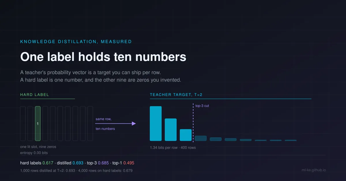
The short version Every supervised dataset ships one integer per row, which is a ten-dimensional vector with nine invented zeros attached. On a task whose labels are ambiguous by construction, an 8-unit student given 400 rows and those one-hot labels reaches 0.617 test accuracy; the same student on the same 400 rows, trained to match a 32-unit teacher’s probability vectors, reaches 0.693, and 4,000 hard-labelled rows still stop at 0.679. The gain survives truncating the target to its top three entries (0.685) and collapses at one (0.495, worse than the plain labels). The second half of this post is the bill: what those targets cost to store, why the temperature exists, and the one regularisation trick that quietly strips the information out.
A hard label answers a question the data cannot answer cleanly. It says this row is class four and not class five, when the annotator, the sensor or the synthetic generator was working with something closer to sixty percent four, thirty percent five and ten percent three. The zeros after the one are not measurements. They are the format.
The fix is old and it is not a model change. Train a larger model once, keep its full probability vector for each row, and hand that vector to the small model instead of the integer. Hinton, Vinyals and Dean described the trade in 2015, and the sentence that carries the argument is theirs:
“When the soft targets have high entropy, they provide much more information per training case than hard targets and much less variance in the gradient between training cases, so the small model can often be trained on much less data than the original cumbersome model and using a much higher learning rate.”
That claim has a specific structure, and the structure is what this post measures. It is not that soft labels are cleaner. It is that one row carries more signal, so the number of rows you need falls. Those are different budgets, and only one of them shows up in your annotation invoice.
A label is one number and nine invented zeros
The information argument is easiest to see in the paper’s own example. A handwritten 2 is sometimes almost a 3 and sometimes almost a 7, and a trained teacher will say so in the tail of its distribution, assigning one 2 a probability of $10^{-6}$ of being a 3 and $10^{-9}$ of being a 7, while another 2 gets the opposite treatment. That ordering is knowledge about which digits resemble which. A one-hot label throws it away.
The paper is also honest about why the tail needs help before it can teach anything:
“This is valuable information that defines a rich similarity structure over the data (i. e. it says which 2’s look like 3’s and which look like 7’s) but it has very little influence on the cross-entropy cost function during the transfer stage because the probabilities are so close to zero.”
Two probabilities of $10^{-6}$ and $10^{-9}$ differ by a factor of a thousand and contribute almost nothing to a loss. Squashing them through a softmax with temperature $T$ is what lifts them into a range where the gradient can see them. So temperature is not a knob for accuracy. It is a magnifying glass for the part of the target that carries the structure, and it has a cost, because it also magnifies the noise the teacher picked up from its own training set.
One note on vocabulary, since it circulates badly. The nickname “dark knowledge” is usually traced to Hinton’s talks; it does not appear in this paper, where a text search for the phrase returns zero hits. The paper’s own words are “the ratios of very small probabilities”. If you are quoting a source, quote what the source says.
What the temperature is buying
The mechanics fit in three lines. The teacher’s logits $z$ become targets $q_i = \exp(z_i/T) / \sum_j \exp(z_j/T)$, the student is trained against those targets with its own logits divided by the same $T$, and the gradient scale needs correcting because softening the distribution shrinks the gradients. Hinton and colleagues state the correction exactly:
“Since the magnitudes of the gradients produced by the soft targets scale as $1/T^2$ it is important to multiply them by $T^2$ when using both hard and soft targets.”
In code that is one multiplication. In practice the term is what keeps the soft-target loss from being swamped by the hard-label loss whenever both are used, and it is easy to leave out because a temperature sweep still produces a curve without it. The demo block below applies it as T * (p - q), which is the gradient of $T^2 \cdot \mathrm{CE}(z/T, q)$ with respect to the student’s logits.
The temperature result people quote most often is the MNIST one, and it is worth having the actual numbers. A network with two hidden layers of 1,200 rectified units, heavily regularised, made 67 test errors. A smaller network with two layers of 800 units and no regularisation made 146. The same smaller network, regularised only by matching the big net’s soft targets at $T = 20$, made 74 errors. The transfer set contained no translated digits, yet the student learned the invariances the teacher had picked up from translation-augmented training. The distilled model also classified 98.6 percent of 3s correctly in a run where every 3 had been removed from its transfer set, once the bias for that class was corrected.
The same paper contains the caveat that most summaries drop. Temperature is not a constant of the method; it depends on how much room the student has:
“When the distilled net had 300 or more units in each of its two hidden layers, all temperatures above 8 gave fairly similar results. But when this was radically reduced to 30 units per layer, temperatures in the range 2.5 to 4 worked significantly better than higher or lower temperatures.”
A small student benefits from partial softening and is hurt by full softening, because at high temperature the target describes a richness the student cannot represent, and the mismatch becomes part of the loss. Cho and Hariharan later made this the centre of their analysis: “larger models do not often make better teachers”, they wrote, and the cause is “mismatched capacity”. Their fix is unglamorous, stopping the teacher’s training early, and they report that the usual workaround of chaining several distillation steps “to be ineffective”.
A task where the ambiguity is real
Most distillation demos are run on tasks where the teacher is nearly deterministic, which makes the whole measurement vacuous: a teacher that outputs one-hot vectors has nothing to transfer beyond the label. The demo below builds a task with real ambiguity and a known ceiling, so the accuracy figures can be read against something other than each other.
Ten classes sit in two groups of five. One feature decides the group. Inside a group the label follows a smooth spread over neighbouring classes, so a row near the boundary of class 2 is genuinely a coin flip between 2 and 3. The generative rule gives the true posterior in closed form, so the reference point is exact rather than another model: the best achievable accuracy on the held-out labels is 0.790, whatever the model size.
The teacher is a 32-unit network trained on 12,000 rows. The student is an 8-unit network trained on 400. Every configuration trains three times with different seeds and the table reports the mean, because single-seed differences of two or three accuracy points in this size class are noise.
Two versions of this experiment failed before the numbers below appeared. The first teacher used a learning rate of 8 and diverged, so the reported “distillation hurts” result was really “the teacher never trained”. The second gave the teacher 15 pure-noise features and 4,000 rows, and it memorised them, so its targets came out effectively one-hot. A demo that cannot show a non-trivial entropy is not measuring distillation.
The measurement
1
2
3
4
5
6
7
8
9
10
11
12
13
14
15
16
17
18
19
20
21
22
23
24
25
26
27
28
29
30
31
32
33
34
35
36
37
38
39
40
41
42
43
44
45
46
47
48
49
50
51
52
53
54
55
56
57
58
59
60
61
62
63
64
65
66
67
68
69
70
71
72
73
74
75
76
77
78
79
80
81
82
83
84
85
86
87
88
89
90
91
92
93
94
95
96
97
98
99
100
101
102
103
104
105
106
import numpy as np

# Task: 10 classes in two groups of five. One feature decides the group; inside
# a group the label follows a smooth spread, so the label is genuinely ambiguous
# given the features. That ambiguity is what a soft target can explain and a
# one-hot label cannot.
C, D = 10, 6
N_TRAIN, N_TEST, N_STUDENT = 12000, 3000, 400

def sample(n, seed):
    rng = np.random.default_rng(seed)
    a = rng.uniform(-1, 1, size=n)
    t = np.abs(a) * 4.5
    p = np.exp(-((t[:, None] - np.arange(5)[None, :])**2) / 0.35)
    p /= p.sum(1, keepdims=True)
    c = (rng.random(n)[:, None] > p.cumsum(1)).sum(1).clip(0, 4)
    y = np.where(a < 0, c, c + 5)
    x = np.column_stack([a + rng.normal(scale=0.05, size=n), rng.normal(size=(n, D - 1))])
    return x, y, a

def posterior(a):                       # the ceiling: true p(class | feature)
    t = np.abs(a) * 4.5
    p = np.exp(-((t[:, None] - np.arange(5)[None, :])**2) / 0.35)
    p /= p.sum(1, keepdims=True)
    out = np.zeros((len(a), C)); neg = a < 0
    out[neg, :5], out[~neg, 5:] = p[neg], p[~neg]
    return out

xtr, ytr, _ = sample(N_TRAIN, 10)
xte, yte, ate = sample(N_TEST, 11)
mu, sd = xtr.mean(0, keepdims=True), xtr.std(0, keepdims=True)
xtr, xte = (xtr - mu) / sd, (xte - mu) / sd

def onehot(y):
    o = np.zeros((len(y), C)); o[np.arange(len(y)), y] = 1.0; return o
def softmax(z):
    z = z - z.max(1, keepdims=True); e = np.exp(z); return e / e.sum(1, keepdims=True)
def entropy(q):
    return float((-(q * np.log2(q + 1e-12)).sum(1)).mean())

class Net:                              # one tanh hidden layer, softmax head
    def __init__(self, h, seed):
        rng = np.random.default_rng(seed)
        self.W1 = rng.normal(scale=1/np.sqrt(D), size=(D, h)); self.b1 = np.zeros(h)
        self.W2 = rng.normal(scale=1/np.sqrt(h), size=(h, C)); self.b2 = np.zeros(C)
        self.p = [self.W1, self.b1, self.W2, self.b2]; self.m = [np.zeros_like(p) for p in self.p]
    def logits(self, x):
        return np.tanh(x @ self.W1 + self.b1) @ self.W2 + self.b2
    def step(self, x, q, T, lr):
        h = np.tanh(x @ self.W1 + self.b1)
        p = softmax((h @ self.W2 + self.b2) / T)     # student logits divided by T
        g = T * (p - q) / len(x)                     # gradient of T^2 * CE(z/T, q)
        gh = (g @ self.W2.T) * (1 - h**2)
        for i, gd in enumerate([x.T @ gh, gh.sum(0), h.T @ g, g.sum(0)]):
            self.m[i] = 0.9 * self.m[i] - lr * gd; self.p[i] += self.m[i]

def fit(x, target, hidden, epochs, lr, seed, T=1.0, batch=64):
    net = Net(hidden, seed); rng = np.random.default_rng(seed + 1)
    for _ in range(epochs):
        idx = rng.permutation(len(x))
        for i in range(0, len(x), batch):
            b = idx[i:i+batch]; net.step(x[b], target[b], T, lr)
    return net

def acc(net, x, y):
    return float((net.logits(x).argmax(1) == y).mean())
def probs(net, x, T=1.0):
    return softmax(net.logits(x) / T)
def topk(q, k):
    out = np.zeros_like(q)
    idx = np.argsort(-q, axis=1)[:, :k]
    np.put_along_axis(out, idx, np.take_along_axis(q, idx, axis=1), axis=1)
    return out / out.sum(1, keepdims=True)           # renormalise what survives

SEEDS = (7, 17, 27)
mean = lambda f, *a, **k: float(np.mean([f(s, *a, **k) for s in SEEDS]))

print(f"posterior ceiling on the test labels    {(posterior(ate).argmax(1) == yte).mean():.3f}")
teacher = fit(xtr, onehot(ytr), 32, 150, 0.3, 3)
print(f"teacher, {N_TRAIN} rows, 32 units        test acc {acc(teacher, xte, yte):.3f}")

xs, ys = xtr[:N_STUDENT], ytr[:N_STUDENT]
print(f"\nstudent, 8 units, {N_STUDENT} rows, mean of 3 seeds")
print(f"  hard labels                      {mean(lambda s: acc(fit(xs, onehot(ys), 8, 300, 0.5, s), xte, yte)):.3f}")
for T in (1, 2, 4, 8):
    q = probs(teacher, xs, T)
    print(f"  soft targets, T={T:<2d}               {mean(lambda s: acc(fit(xs, q, 8, 300, 0.5, s, T=T), xte, yte)):.3f}"
          f"   labels {entropy(q):.2f} bits")

qb = probs(teacher, xs, 2)
print("\nsame student, the top k of the T=2 targets, renormalised")
for k in (1, 2, 3, 5, 10):
    print(f"  k={k:<2d}                            {mean(lambda s: acc(fit(xs, topk(qb, k), 8, 300, 0.5, s, T=2), xte, yte)):.3f}")

smoothed = fit(xtr, 0.9 * onehot(ytr) + 0.1 / C, 32, 150, 0.3, 3)
qs = probs(smoothed, xs, 2)
print(f"\nteacher trained with label smoothing 0.1")
print(f"  teacher test acc                 {acc(smoothed, xte, yte):.3f}")
print(f"  student on its T=2 targets       {mean(lambda s: acc(fit(xs, qs, 8, 300, 0.5, s, T=2), xte, yte)):.3f}")

soft_all = probs(teacher, xtr, 2)
print("\nlabel budget: hard labels vs the same rows distilled at T=2")
for n in (400, 1600, 4000):
    h = mean(lambda s: acc(fit(xtr[:n], onehot(ytr[:n]), 8, 300, 0.5, s), xte, yte))
    d = mean(lambda s: acc(fit(xtr[:n], soft_all[:n], 8, 300, 0.5, s, T=2), xte, yte))
    print(f"  {n:5d} rows    hard {h:.3f}    distilled {d:.3f}")
1
2
3
4
5
6
7
8
9
10
11
12
13
14
15
16
17
18
19
20
21
22
23
24
25
posterior ceiling on the test labels    0.790
teacher, 12000 rows, 32 units        test acc 0.683

student, 8 units, 400 rows, mean of 3 seeds
  hard labels                      0.617
  soft targets, T=1                0.685   labels 0.93 bits
  soft targets, T=2                0.693   labels 1.34 bits
  soft targets, T=4                0.651   labels 1.79 bits
  soft targets, T=8                0.616   labels 2.35 bits

same student, the top k of the T=2 targets, renormalised
  k=1                             0.495
  k=2                             0.589
  k=3                             0.685
  k=5                             0.694
  k=10                            0.693

teacher trained with label smoothing 0.1
  teacher test acc                 0.692
  student on its T=2 targets       0.692

label budget: hard labels vs the same rows distilled at T=2
    400 rows    hard 0.617    distilled 0.693
   1600 rows    hard 0.660    distilled 0.685
   4000 rows    hard 0.679    distilled 0.689
Reading the temperature column
The first thing the table shows is that the exercise is not free: the teacher reaches 0.683 and the ceiling is 0.790, so about 11 accuracy points are the teacher’s own shortfall and no student can recover them. A teacher trained longer or wider would move that wall, and the student’s ceiling moves with it. This is the property that makes distillation a budget rather than a trick: what transfers is what the teacher knows, minus what the student can represent.
The second thing is the shape. Distillation at $T=1$ is already worth 6.8 points over the hard labels. It peaks at $T=2$, worth 7.6 points, which is the point where the target has 1.34 bits of entropy per row and the second and third classes sit in a range the 8-unit student can use. By $T=4$ the entropy is 1.79 bits and accuracy has fallen back to 0.651. At $T=8$ it is 2.35 bits, and the student is below where it started: 0.616 against 0.617 for plain labels.
That last row is the one to keep, because it is the failure mode you will hit first if you copy a temperature from a paper. A high temperature flattens the target toward uniform, and once the target is mostly uniform the student is being asked to match the teacher’s uncertainty about everything, including the noise. The published guidance and the measurement agree: intermediate temperatures for small students, and the student’s capacity decides what counts as intermediate, not the teacher’s.
The label-budget rows make the economic case better than the accuracy columns do, because they compare the two things distillation is supposed to trade. Four hundred distilled rows reach 0.693. Hard labels need 4,000 rows to reach 0.679, and the 8-unit student appears to flatten there, which is its capacity ceiling rather than a shortage of data. Ten times the label spend loses to the same 400 rows plus a teacher, and the margin is not close.
Where truncation starts to cost you
Shipping a teacher’s probability vector for every row is a storage decision, so the honest question is how much of the vector you can cut before the gain goes with it. The run renormalises the surviving top $k$ entries and trains the same student.
The result is not gradual. Keeping only the largest entry, which is the teacher’s argmax renormalised to 1.0, is exactly the pseudo-labelling recipe: take the teacher’s best guess and train on it as if it were a label. That scores 0.495, well below the 0.617 the student gets from 400 human labels. The teacher is 68 percent accurate on this task, and pseudo-labels import its errors with the same confidence as its successes. Keeping two entries recovers 0.589, still below plain labels. Keeping three reaches 0.685, within noise of the full vector’s 0.693. Five and ten add nothing measurable.
So the first cut that keeps the gain is three, and the mechanism explains why. A two-entry target still cannot represent the three-class spread the task generates, and renormalising two probabilities into a corner distorts the ratio the student is trying to learn. Three entries can hold the local structure. In a ten-class problem that is 30 percent of the row; the next block prices it at the scale where the question bites.
1
2
3
4
5
6
7
8
9
10
11
12
13
14
15
16
17
18
19
20
21
22
ROWS = 1_000_000

def human(total):
    for unit, div in (("GB", 1e9), ("MB", 1e6), ("KB", 1e3)):
        if total >= div:
            return f"{total/div:.1f} {unit}"
    return f"{total:.0f} B"

size = lambda per_row: human(per_row * ROWS)

print(f"targets for {ROWS:,} training rows, float16 everywhere")
print(f"{'vocab':>7s} {'full':>12s} {'top-3':>10s} {'top-8':>10s} {'top-8 vs full':>14s}")
for vocab in (10, 1000, 32768, 128000):
    full = vocab * 2                    # one float16 probability per class
    t3 = min(3, vocab) * 4              # float16 probability + uint16 class id
    t8 = min(8, vocab) * 4
    print(f"{vocab:>7d} {size(full):>12s} {size(t3):>10s} {size(t8):>10s} {full/t8:>13.1f}x")

print()
print(f"this post's 10-class task, one row of full targets: {10*2} bytes")
print(f"12,000 rows of full targets: {human(12000*20)}")
print(f"top-3 of 10 classes: {3*4} bytes, {10*2/(3*4):.1f}x smaller")
1
2
3
4
5
6
7
8
9
10
targets for 1,000,000 training rows, float16 everywhere
  vocab         full      top-3      top-8  top-8 vs full
     10      20.0 MB    12.0 MB    32.0 MB           0.6x
   1000       2.0 GB    12.0 MB    32.0 MB          62.5x
  32768      65.5 GB    12.0 MB    32.0 MB        2048.0x
 128000     256.0 GB    12.0 MB    32.0 MB        8000.0x

this post's 10-class task, one row of full targets: 20 bytes
12,000 rows of full targets: 240.0 KB
top-3 of 10 classes: 12 bytes, 1.7x smaller
Read the ten-class line first, because it shows truncation is not automatically a saving. With ten classes a full float16 vector is 20 bytes and a top-8 target is 32, since each retained entry now stores an identifier alongside its probability. Sparse targets only pay when the vocabulary is much larger than the cut, and that condition holds for language models and almost nothing else. At a 32,768-token vocabulary the full row is 65.5 GB per million training rows and top-8 is 32 MB, a factor of 2,048. At 128,000 tokens it is 256 GB against the same 32 MB.
This is the real constraint behind logit-based distillation of language models, and it is why the published methods at that scale either keep a cut over the vocabulary or compute the divergence on the student’s own generated sequences instead of on a stored target table.
The smoothing trap that fires in one direction
Label smoothing is a common way to train a teacher, and Müller, Kornblith and Hinton found the reason to be careful about combining it with distillation:
“if a teacher network is trained with label smoothing, knowledge distillation into a student network is much less effective.”
Their explanation is precisely the information this post has been measuring: smoothing pulls a class’s examples into tight clusters, which “results in loss of information in the logits about resemblances between instances of different classes, which is necessary for distillation”.
I expected to reproduce that damage and did not. In this task the smoothed teacher scored 0.692 on its own, slightly better than the 0.683 of the unsmoothed one, and its student reached 0.692 against 0.693. The honest reading is that my task’s between-class structure is coarse, two groups of five with a smooth spread inside each, so flattening the distribution by a tenth removes little that the student was using. Müller and colleagues were working with fine-grained image classes where the resemblance structure is the point.
Report the negative result rather than trimming it, because the practical rule survives it: whether smoothing costs you anything is an empirical question about your teacher and label geometry, and it is a one-line experiment. What the published result establishes is the direction of the risk, and the risk is one-way: smoothing can remove information from the target, never add it.
What this costs at language-model scale
The same arithmetic runs at the scale where distillation is now routine, with one wrinkle the classification demo does not have. For autoregressive models the student is trained on sequences, and sequences that the teacher would produce are not the sequences in the dataset, so matching a stored target table on the training corpus optimises the wrong distribution. Agarwal and colleagues name the problem and the fix in their description of generalised knowledge distillation: current methods “suffer from distribution mismatch between output sequences seen during training and those generated by the student during inference”, and their answer is to let the student generate and have the teacher score those generations. Gu and colleagues take the same observation in a different direction, replacing the forward Kullback-Leibler divergence with the reverse one so the student stops “overestimating the low-probability regions of the teacher distribution”, and report results from 120M to 13B parameters.
The industrial evidence is easier to check than the papers, because the artifacts are on the Hub. DistilBERT established the pattern for encoders: 40 percent smaller, 97 percent of the language understanding, 60 percent faster, with a triple loss combining language modelling, distillation and a cosine-distance term. On the decoder side, DeepSeek’s R1 distilled models are a public example of the budget this post has been pricing: the 7B Qwen-derived checkpoint is listed at 7,615,616,512 parameters under an MIT licence, first published on 20 January 2025, with roughly 298,000 downloads and 962 likes at the time of checking.
Those releases show that the choice this post measures, how much of the teacher’s distribution to keep, is not academic bookkeeping. A full logit table at 128,000 vocabulary tokens is 256 GB per million rows, so practical recipes keep a cut, generate the targets on the fly, or use a divergence that never materialises the table. The top-3 finding here is the small-scale version of that decision: find the cut where the structure stops fitting, and stop there.
A protocol you can run this week
- Measure the teacher’s entropy before anything else. Compute the mean entropy of its targets on a held-out slice. If it is under 0.1 bits on a ten-class problem, you have a pseudo-labeller, not a teacher, and the rest of the recipe will not help.
- Sweep temperature against the student’s capacity, not the teacher’s. Three values, $T \in {1, 2, 4}$, three seeds, mean and spread. If the best value is at the edge of your grid, extend it; if the curve is flat, the student already fits.
- Cut the target by measurement. Start at $k = 3$ for classification. Going to $k = 1$ is a different technique with a different failure mode, and on a 68-percent teacher it lost 12 points against the labels it replaced.
- Keep $T^2$ in the loss. If you combine soft and hard terms, the missing factor shows up as the hard term dominating at high temperature, which reads like “soft labels do not help” in the ablations.
- Do not label-smooth the teacher unless you test both. The published result says the target loses inter-class resemblance; my measurement says the size of the loss depends on your class geometry. It is one extra training run to know.
- Price the targets before you commit. Full float16 logits at 32,768 tokens is 65.5 GB per million rows. If that is a hard no for your pipeline, decide the cut now rather than after the teacher is trained.
The step most teams skip is the first. A distillation run whose teacher has not been checked for entropy is a run whose result cannot be interpreted: it may have transferred structure, or it may have transferred a confident wrong answer four hundred times.
Key takeaways
| What looks like the answer | What it is | What to do instead |
|---|---|---|
| The label on each row | A ten-dimensional target with nine zeros nobody measured | Ship the teacher’s probability vector, or its top few entries |
| More rows will close the gap | Distillation at 400 rows beat hard labels at 4,000, and the student had flattened out | Spend on the teacher once, then reuse it across students |
| Higher temperature is more information | Entropy rises from 1.34 to 2.35 bits between $T=2$ and $T=8$, and accuracy falls from 0.693 to 0.616 | Sweep temperature against student capacity, keep the $T^2$ factor |
| Top-1 distill is a cheap approximation | It is pseudo-labelling: 0.495 against 0.617 for the labels it replaced | Keep at least three entries, or keep the label |
| Label smoothing is free | It can only remove resemblance information from the target | Train the teacher both ways before choosing |
| Full logits everywhere | 65.5 GB per million rows at a 32,768-token vocabulary | Cut by measurement, or generate targets on the fly |
The demo is synthetic and seeded, and the numbers are there to make the arithmetic visible rather than to publish a benchmark. What transfers is the shape: soft targets buy label efficiency, the gain peaks at a temperature set by the student, it survives a small cut, and it dies at a cut of one.
References
- Hinton, Vinyals & Dean, Distilling the Knowledge in a Neural Network, 2015 — https://arxiv.org/abs/1503.02531
- Cho & Hariharan, On the Efficacy of Knowledge Distillation, 2019 — https://arxiv.org/abs/1910.01348
- Müller, Kornblith & Hinton, When Does Label Smoothing Help?, NeurIPS 2019 — https://arxiv.org/abs/1906.02629
- Sanh, Debut, Chaumond & Wolf, DistilBERT, a distilled version of BERT, 2019 — https://arxiv.org/abs/1910.01108
- Agarwal, Vieillard, Zhou, Stanczyk, Ramos, Geist & Bachem, On-Policy Distillation of Language Models: Learning from Self-Generated Mistakes, ICLR 2024 — https://arxiv.org/abs/2306.13649
- Gu, Dong, Wei & Huang, MiniLLM: Knowledge Distillation of Large Language Models, ICLR 2024 — https://arxiv.org/abs/2306.08543
- DeepSeek-R1-Distill-Qwen-7B model card, 7,615,616,512 parameters, MIT licence, published 20 January 2025 — https://huggingface.co/deepseek-ai/DeepSeek-R1-Distill-Qwen-7B
Related posts
- How Many Labels Does Your Language Need? Build the Curve Before You Buy — the row-count budget this post converts into a per-row information budget
- Rank Is a Budget: What LoRA at r=8 Costs and Buys on an 8B Model — the student-side capacity knob that sets the useful temperature
- Cascade Routing: Pay for the Big Model Only on the Queries That Need It — the alternative to compressing the teacher, routing to it instead
- Is Your +3-Point Eval Gain Real? Gating a Comparison with Paired Statistics — how to test a 7.6-point difference properly across seeds
- Pass@k and Reliability: What a Score Means Across Attempts — why one accuracy figure rarely settles a comparison