Clicks Are Not Judgments: Debiasing Retrieval Feedback with Inverse Propensity Weights
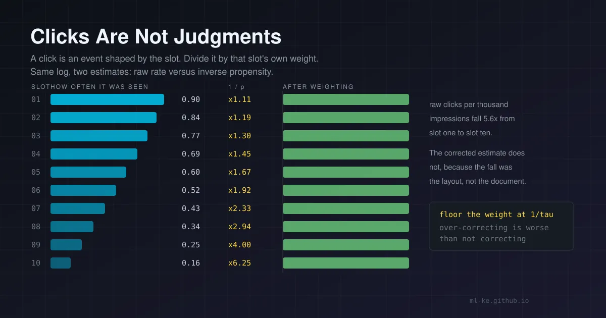
The short version Click logs are the cheapest relevance signal a retrieval team has, and they are a measurement of two things at once: what users wanted and where your ranker put the document. Reading them at face value gives an estimate that tracks your own ranking policy. In a seeded simulation where the truth is known, the raw click rate puts 15 relevance points on the floor and 64 times more traffic removes 4 percent of that error, while inverse propensity weighting cuts the gap to 2 points and drops the top-ten NDCG error from 0.099 to 0.019. The correction has its own failure modes, and this post measures those too.
You shipped a retrieval change last month and the logs have been talking ever since. Passage seven gets clicked four times more than passage twelve, so seven goes first. A quarter later the search quality metric has not moved, the click pattern looks exactly like the old one, and someone asks whether users just click whatever is on top.
They do. That is not a mystery of user behaviour, it is arithmetic you can put a number on.
Four recent posts build the measurement stack around retrieval: paired statistics for deciding whether a difference is real, recall at k for reading the metric’s denominator honestly, pass@k reliability for what a score means across attempts, and rank fusion for combining two retrievers. Each assumes the labels are labels. This post is about the case where the label is a click, which is not a judgment but an event that depends on where you put the document.
The log records two things and you only want one
The clearest evidence is twenty years old and still the best illustration. Joachims, Granka, Pan, Hembrooke and Gay put an eye-tracker on people using Google and recorded which abstracts they actually looked at before they clicked. Their Table 2 reports, for each click position, the percentage of sessions where the user had viewed the abstract at each rank above it: before a click on link three, users had viewed abstract one 73.9 percent of the time and abstract two 82.6 percent of the time. Their summary of the display is the sentence to keep:
“It is very interesting that users click substantially more often on the first than on the second link, while they view the corresponding abstract with almost equal frequency.”
That is the whole confound in one line. If attention were uniform, click counts would compare documents. Because attention falls with rank, click counts compare positions.
The published numbers are blunt about how fast attention decays. In the same table, the rank-one abstract was viewed in 90.6 percent of sessions where the click landed on rank one, and the rank-six abstract in 4.3 percent. Wang, Bendersky, Metzler and Najork measured the same thing as a click propensity on a commercial email search product: position one carried about 0.40 of the click mass, position four about 0.15. They also measured a second corpus in the same study whose profile was much flatter, the first hint that you cannot borrow a propensity table from a paper and use it on your product.
What the naive rate actually estimates
Write the click as the product of two events. A user examines the document, which depends on the slot, and then clicks it, which depends on whether the document answers the query. Under the position-based model the two factors separate:
\[P(\text{click}_{d} \mid \text{slot}=r) = p_r \cdot \text{rel}_d\]The simulation below reproduces this with one extra detail: clicks are noisy, so a grade-3 document is clicked 90 percent of the time it is examined, a grade-1 document 20 percent, a grade-0 document never.
Once the factorization is on the page, the failure of the raw click rate is not subtle. Clicks over impressions estimates $p_r \cdot \text{rel}_d$ averaged over the slots a document happened to occupy, and that average is a property of your ranker, not of the document. Two consequences follow, both measurable:
- The estimate is biased low by roughly the average examination propensity, so every document in the catalogue looks worse than it is.
- The bias is not uniform. Documents your ranker buries are examined least, so their estimates are dragged down hardest, which is precisely the set of documents a retrieval improvement is supposed to surface.
The fix is inverse propensity weighting: divide each click by the propensity of the slot it happened in, and the position factor cancels in expectation.
\[\hat{r}_d = \frac{1}{n_d} \sum_{i \in \text{impressions}(d)} \frac{c_{di}}{p_{\text{slot}(d,i)}}\]Joachims, Swaminathan and Schnabel give the condition that makes this work in their derivation: the estimator is unbiased only if $p_r > 0$ for every rank. The moment a slot cannot be examined at all, no reweighting recovers what happened there. Keep that constraint in mind, because it is the hard limit at the end of the post.
The demo: one log, two estimators
The simulation fixes the truth, which is the only way to score an estimator rather than an outcome. One hundred and twenty documents each carry a graded relevance and an incumbent score that is independent of relevance. Thirty thousand impressions come from ranking fifteen candidates and showing the top ten, and a click arrives only when a document is examined and then judged good. Every seed feeds both estimators the same log.
1
2
3
4
5
6
7
8
9
10
11
12
13
14
15
16
17
18
19
20
21
22
23
24
25
26
27
28
29
30
31
32
33
34
35
36
37
38
39
40
41
42
43
44
45
46
47
48
49
50
51
52
53
54
55
56
57
58
59
60
61
62
63
64
65
66
import math, random

CAND, SLOTS, DOCS, QUERIES = 15, 10, 120, 3000
# examination propensity by rank: the shape the eye-tracking study reports
P_EXAM = [0.90, 0.84, 0.77, 0.69, 0.60, 0.52, 0.43, 0.34, 0.25, 0.16]
CLICK_RATE = [0.0, 0.20, 0.55, 0.90]        # P(click | examined, relevance grade)

def simulate(seed):
    rng = random.Random(seed)
    grade = rng.choices([0, 1, 2, 3], weights=[45, 25, 20, 10], k=DOCS)
    logger = [rng.random() for _ in range(DOCS)]   # incumbent score, unrelated to relevance
    shown, clicks, weighted = [0]*DOCS, [0]*DOCS, [0.0]*DOCS
    for _ in range(QUERIES):
        pool = sorted(rng.sample(range(DOCS), CAND), key=lambda d: -logger[d])
        for pos, d in enumerate(pool[:SLOTS]):
            shown[d] += 1
            if rng.random() < P_EXAM[pos] and rng.random() < CLICK_RATE[grade[d]]:
                clicks[d] += 1
                weighted[d] += 1.0 / P_EXAM[pos]
    truth = [CLICK_RATE[g] for g in grade]
    safe = lambda n, d: n / d if d else 0.0
    naive = [safe(clicks[d], shown[d]) for d in range(DOCS)]
    ips = [safe(weighted[d], shown[d]) for d in range(DOCS)]
    return truth, naive, ips, grade, shown, logger

def spearman(xs, ys):
    n = len(xs)
    def ranks(v):
        idx = sorted(range(n), key=lambda i: v[i]); out = [0.0]*n; i = 0
        while i < n:
            j = i
            while j + 1 < n and v[idx[j+1]] == v[idx[i]]:
                j += 1
            for k in range(i, j+1):
                out[idx[k]] = (i + j) / 2.0
            i = j + 1
        return out
    a, b = ranks(xs), ranks(ys)
    ma, mb = sum(a)/n, sum(b)/n
    return (sum((a[i]-ma)*(b[i]-mb) for i in range(n))
            / math.sqrt(sum((x-ma)**2 for x in a) * sum((y-mb)**2 for y in b)))

def ndcg(order, grade):
    dcg = sum(grade[d] / math.log2(i + 2) for i, d in enumerate(order[:SLOTS]))
    ideal = sorted(grade, reverse=True)
    return dcg / sum(ideal[i] / math.log2(i + 2) for i in range(SLOTS))

runs = [simulate(s) for s in range(8)]
mean = lambda f: sum(f(r) for r in runs) / len(runs)
rmse = lambda e, t: math.sqrt(sum((e[d]-t[d])**2 for d in range(DOCS)) / DOCS)
bias = lambda e, t: sum(e[d]-t[d] for d in range(DOCS)) / DOCS
top = lambda v: sorted(range(DOCS), key=lambda d: -v[d])

print(f"{DOCS} documents, {QUERIES} queries, mean of 8 seeds")
print(f"{'estimator':10s}{'rho':>7s}{'NDCG@10':>9s}{'RMSE':>8s}{'bias':>8s}")
for name, i in (("naive CTR", 1), ("IPS", 2)):
    print(f"{name:10s}{mean(lambda r, i=i: spearman(r[i], r[0])):7.3f}"
          f"{mean(lambda r, i=i: ndcg(top(r[i]), r[3])):9.3f}"
          f"{mean(lambda r, i=i: rmse(r[i], r[0])):8.3f}"
          f"{mean(lambda r, i=i: bias(r[i], r[0])):8.3f}")

print(f"\ncorrelation with the incumbent's own score")
print(f"  naive estimate      {mean(lambda r: spearman(r[1], r[5])):+.3f}")
print(f"  IPS estimate        {mean(lambda r: spearman(r[2], r[5])):+.3f}")
print(f"  true relevance      {mean(lambda r: spearman(r[0], r[5])):+.3f}")
print(f"\ndocuments never shown: {sum(1 for s in runs[0][4] if s == 0)} of {DOCS}")
The output:
1
2
3
4
5
6
7
8
9
10
11
120 documents, 3000 queries, mean of 8 seeds
estimator     rho  NDCG@10    RMSE    bias
naive CTR   0.845    0.901   0.253  -0.150
IPS         0.869    0.981   0.186  -0.021

correlation with the incumbent's own score
  naive estimate      +0.396
  IPS estimate        +0.251
  true relevance      +0.077

documents never shown: 11 of 120
Read the correlation block first, because it measures the confound directly. The raw click rate lines up with the incumbent’s own score at 0.396, five times more strongly than true relevance does at 0.077. The estimator has absorbed the ranker’s opinion, and that opinion is not the one you were trying to measure. IPS drops the association to 0.251.
The ranking numbers show what that costs. Relevance order goes from 0.845 to 0.869, which sounds small until you read NDCG@10: 0.901 against 0.981. Spearman averages over the whole catalogue; NDCG@10 is the list a user sees, and the raw click rate mis-assembles its top by ten points.
Mean signed bias falls from −0.150 to −0.021. That first number deserves a beat: every document looks about fifteen points less relevant than it is, on a scale where a fully relevant document scores 0.90. More traffic does not remove that gap, which is the subject of the next section.
More traffic does not remove bias
The instinct when an estimate looks noisy is to wait for more clicks. Bias does not care how long you wait. Variance does.
The next block reruns the same generator at four traffic levels and reports the two error components separately.
1
2
3
4
5
6
7
8
9
10
11
12
13
14
15
16
17
18
19
20
21
22
23
24
25
26
27
28
29
30
31
32
33
34
35
36
37
import math, random

CAND, SLOTS, DOCS = 15, 10, 120
P_EXAM = [0.90, 0.84, 0.77, 0.69, 0.60, 0.52, 0.43, 0.34, 0.25, 0.16]
CLICK_RATE = [0.0, 0.20, 0.55, 0.90]

def simulate(seed, queries):
    rng = random.Random(seed)
    grade = rng.choices([0, 1, 2, 3], weights=[45, 25, 20, 10], k=DOCS)
    logger = [rng.random() for _ in range(DOCS)]
    shown, clicks, weighted = [0]*DOCS, [0]*DOCS, [0.0]*DOCS
    for _ in range(queries):
        pool = sorted(rng.sample(range(DOCS), CAND), key=lambda d: -logger[d])
        for pos, d in enumerate(pool[:SLOTS]):
            shown[d] += 1
            if rng.random() < P_EXAM[pos] and rng.random() < CLICK_RATE[grade[d]]:
                clicks[d] += 1
                weighted[d] += 1.0 / P_EXAM[pos]
    truth = [CLICK_RATE[g] for g in grade]
    safe = lambda n, d: n / d if d else 0.0
    return (truth,
            [safe(clicks[d], shown[d]) for d in range(DOCS)],
            [safe(weighted[d], shown[d]) for d in range(DOCS)])

rmse = lambda est, truth: math.sqrt(sum((est[d]-truth[d])**2 for d in range(DOCS)) / DOCS)
bias = lambda est, truth: sum(est[d]-truth[d] for d in range(DOCS)) / DOCS

print("bias and error against query volume (8 seeds, mean)")
print(f"{'queries':>8s}{'naive RMSE':>12s}{'naive bias':>12s}{'IPS RMSE':>10s}{'IPS bias':>10s}")
for queries in (300, 1200, 4800, 19200):
    runs = [simulate(s, queries) for s in range(8)]
    mean = lambda f: sum(f(r) for r in runs) / len(runs)
    print(f"{queries:8d}"
          f"{mean(lambda r: rmse(r[1], r[0])):12.3f}"
          f"{mean(lambda r: bias(r[1], r[0])):12.3f}"
          f"{mean(lambda r: rmse(r[2], r[0])):10.3f}"
          f"{mean(lambda r: bias(r[2], r[0])):10.3f}")
1
2
3
4
5
6
bias and error against query volume (8 seeds, mean)
 queries  naive RMSE  naive bias  IPS RMSE  IPS bias
     300       0.260      -0.150     0.268    -0.029
    1200       0.255      -0.151     0.175    -0.025
    4800       0.251      -0.149     0.182    -0.016
   19200       0.250      -0.149     0.152    -0.015
Sixty-four times the traffic moves the naive error from 0.260 to 0.250, a four percent reduction, while its bias does not move: −0.150, −0.151, −0.149, −0.149. The corrected estimator’s error falls from 0.268 to 0.152 over the same range, because what it has left to lose is sampling noise, and sampling noise is the part that averages out.
A team with a small log and an honest estimator should expect wide error bars. A team with an enormous log and a naive estimator should expect tight error bars around a number that is wrong, which is worse, because tight error bars are what gets a number into a dashboard without a follow-up question.
Clipping is a decision about variance
Inverse weighting buys unbiasedness by multiplying small propensities into large weights. A click at slot ten with a propensity of 0.16 contributes 6.25 to a document’s sum, so a document that was seen eleven times and clicked once at the bottom of the list can outrank a document that was seen four hundred times and clicked ninety times. That is the variance the correction imports.
The standard control is a floor on the propensity, which caps the weight at $1/\tau$. Joachims and colleagues describe it as clipping small propensities to a threshold “to trade bias for variance,” and they cross-validate $\tau$ rather than fixing it. Clipping is conservative in a specific sense: it overestimates the propensity of buried slots, so it leaves some of the bias in place and removes the extreme weights.
1
2
3
4
5
6
7
8
9
10
11
12
13
14
15
16
17
18
19
20
21
22
23
24
25
26
27
28
29
30
31
32
33
34
35
36
37
38
39
40
41
42
43
44
45
46
47
import math, random

CAND, SLOTS, DOCS, QUERIES = 15, 10, 120, 3000
P_EXAM = [0.90, 0.84, 0.77, 0.69, 0.60, 0.52, 0.43, 0.34, 0.25, 0.16]
CLICK_RATE = [0.0, 0.20, 0.55, 0.90]

def simulate(seed):
    rng = random.Random(seed)
    grade = rng.choices([0, 1, 2, 3], weights=[45, 25, 20, 10], k=DOCS)
    logger = [rng.random() for _ in range(DOCS)]
    shown = [0]*DOCS
    hit_positions = [[] for _ in range(DOCS)]
    for _ in range(QUERIES):
        pool = sorted(rng.sample(range(DOCS), CAND), key=lambda d: -logger[d])
        for pos, d in enumerate(pool[:SLOTS]):
            shown[d] += 1
            if rng.random() < P_EXAM[pos] and rng.random() < CLICK_RATE[grade[d]]:
                hit_positions[d].append(pos)
    truth = [CLICK_RATE[g] for g in grade]
    def estimate(floor):
        out = []
        for d in range(DOCS):
            if shown[d] == 0:
                out.append(0.0)
            else:
                out.append(sum(1.0 / max(P_EXAM[p], floor) for p in hit_positions[d]) / shown[d])
        return out
    return truth, estimate(0.0), estimate(0.2), estimate(0.3), estimate(0.4), estimate(0.5), grade

def ndcg(order, grade):
    dcg = sum(grade[d] / math.log2(i + 2) for i, d in enumerate(order[:SLOTS]))
    ideal = sorted(grade, reverse=True)
    return dcg / sum(ideal[i] / math.log2(i + 2) for i in range(SLOTS))

rmse = lambda est, truth: math.sqrt(sum((est[d]-truth[d])**2 for d in range(DOCS)) / DOCS)
bias = lambda est, truth: sum(est[d]-truth[d] for d in range(DOCS)) / DOCS
top = lambda v: sorted(range(DOCS), key=lambda d: -v[d])

runs = [simulate(s) for s in range(8)]
mean = lambda f: sum(f(r) for r in runs) / len(runs)
print("propensity floor: weights capped at 1/floor")
print(f"{'floor':>7s}{'RMSE':>8s}{'bias':>8s}{'NDCG@10':>9s}")
for floor, i in ((0.0, 1), (0.2, 2), (0.3, 3), (0.4, 4), (0.5, 5)):
    label = "none" if floor == 0 else f"{floor:.1f}"
    print(f"{label:>7s}{mean(lambda r, i=i: rmse(r[i], r[0])):8.3f}"
          f"{mean(lambda r, i=i: bias(r[i], r[0])):8.3f}"
          f"{mean(lambda r, i=i: ndcg(top(r[i]), r[6])):9.3f}")
1
2
3
4
5
6
7
propensity floor: weights capped at 1/floor
  floor    RMSE    bias  NDCG@10
   none   0.186  -0.021    0.981
    0.2   0.171  -0.032    0.984
    0.3   0.163  -0.051    0.981
    0.4   0.172  -0.069    0.969
    0.5   0.186  -0.085    0.946
The trade shows up where the theory says it will. Bias grows monotonically as the floor rises, from −0.021 to −0.085, because a higher floor under-corrects the bottom of the list. Error does not: it falls to 0.163 at a floor of 0.3 and climbs back to 0.186 at 0.5. Choose the floor that minimizes error, not the one that minimizes bias, and here that sits about a fifth of the way from the minimum propensity (0.16) to the top one (0.90).
A floor does a second job on a real catalogue. A click at slot ten carries a weight of 6.25, so a document with two impressions and one lucky click scores above 3 against a maximum possible relevance of 0.90. A heavy-tailed weight distribution like that makes the top of your ranking unstable across retrains; the floor bounds it at a price you measured rather than guessed.
Where the profile comes from
Nothing above works without $p_r$, and the honest answer is that you do not know it. You estimate it, and the standard way costs traffic.
Wang and colleagues permute the results uniformly at random and show the shuffled list “to a small fraction of end users,” then read the propensity off the click distribution in that slice. Joachims and colleagues took the cheaper version: for seven days their live arXiv search engine swapped the top document with a landmark rank, and they collected clicks on the swapped lists to fit a position-based profile. The delivered model then beat their production ranker in an interleaving experiment, 87 wins against 48 losses and 83 ties, a two-tailed sign test at p = 0.001.
The randomized slice has to be genuinely randomized, and that is a product cost, not just an engineering one. Ai, Bi, Guo and Croft note the objection to swap-based collection directly: it “introduces non-deterministic ranking functions into the product system” and “may hurt the user experience by putting more irrelevant documents on the top.” Their alternative is to learn the propensities jointly with the ranker from ordinary click logs, which avoids the intervention but inherits its own identifiability problems.
A useful middle path, and the one I would start with: randomize a small, fixed share of traffic, estimate the profile from that slice, and freeze it until the ranking template changes. Propensities belong to layouts. Ten slots becoming a grid, a new sidebar, a different snippet length, a mobile-only template: each one moves them, and a profile learned on last quarter’s page measures a page that no longer exists. That is what the email-versus-files comparison really shows: two corpora, one product, two profiles.
How wrong can the profile be
If you cannot measure the profile exactly, the question becomes how much the estimate degrades when the profile is wrong. The next block replaces the true profile $p_r$ with $p_r^{\gamma}$: $\gamma = 0$ assumes no position effect at all, $\gamma = 1$ is the truth, and $\gamma > 1$ exaggerates it.
1
2
3
4
5
6
7
8
9
10
11
12
13
14
15
16
17
18
19
20
21
22
23
24
25
26
27
28
29
30
31
32
33
34
35
36
37
38
39
40
41
42
43
44
45
46
import math, random

CAND, SLOTS, DOCS, QUERIES = 15, 10, 120, 3000
P_EXAM = [0.90, 0.84, 0.77, 0.69, 0.60, 0.52, 0.43, 0.34, 0.25, 0.16]
CLICK_RATE = [0.0, 0.20, 0.55, 0.90]

def simulate(seed):
    rng = random.Random(seed)
    grade = rng.choices([0, 1, 2, 3], weights=[45, 25, 20, 10], k=DOCS)
    logger = [rng.random() for _ in range(DOCS)]
    shown = [0]*DOCS
    hit_positions = [[] for _ in range(DOCS)]
    for _ in range(QUERIES):
        pool = sorted(rng.sample(range(DOCS), CAND), key=lambda d: -logger[d])
        for pos, d in enumerate(pool[:SLOTS]):
            shown[d] += 1
            if rng.random() < P_EXAM[pos] and rng.random() < CLICK_RATE[grade[d]]:
                hit_positions[d].append(pos)
    truth = [CLICK_RATE[g] for g in grade]
    safe = lambda n, d: n / d if d else 0.0
    naive = [safe(len(hit_positions[d]), shown[d]) for d in range(DOCS)]
    def estimate(gamma):          # p' = p ** gamma; gamma=0 assumes no position effect
        return [safe(sum(P_EXAM[p] ** -gamma for p in hit_positions[d]), shown[d])
                for d in range(DOCS)]
    return truth, naive, {g: estimate(g) for g in (0.0, 0.5, 1.0, 1.5)}, grade

runs = [simulate(s) for s in range(8)]
rmse = lambda e, t: math.sqrt(sum((e[d]-t[d])**2 for d in range(DOCS)) / DOCS)
bias = lambda e, t: sum(e[d]-t[d] for d in range(DOCS)) / DOCS
top = lambda v: sorted(range(DOCS), key=lambda d: -v[d])
def ndcg(order, grade):
    dcg = sum(grade[d] / math.log2(i + 2) for i, d in enumerate(order[:SLOTS]))
    ideal = sorted(grade, reverse=True)
    return dcg / sum(ideal[i] / math.log2(i + 2) for i in range(SLOTS))

mean = lambda f: sum(f(r) for r in runs) / len(runs)
print("assumed propensity profile p**gamma; the true profile is gamma = 1")
print(f"{'gamma':>6s}{'RMSE':>8s}{'bias':>8s}{'NDCG@10':>9s}")
for g in (0.0, 0.5, 1.0, 1.5):
    print(f"{g:6.1f}{mean(lambda r, g=g: rmse(r[2][g], r[0])):8.3f}"
          f"{mean(lambda r, g=g: bias(r[2][g], r[0])):8.3f}"
          f"{mean(lambda r, g=g: ndcg(top(r[2][g]), r[3])):9.3f}")

identical = all(abs(a - b) < 1e-12 for truth, naive, est, grade in runs
                for a, b in zip(est[0.0], naive))
print(f"gamma = 0 reproduces the raw click rate exactly: {identical}")
1
2
3
4
5
6
7
assumed propensity profile p**gamma; the true profile is gamma = 1
 gamma    RMSE    bias  NDCG@10
   0.0   0.253  -0.150    0.901
   0.5   0.198  -0.104    0.948
   1.0   0.186  -0.021    0.981
   1.5   0.479   0.144    0.900
gamma = 0 reproduces the raw click rate exactly: True
The first line closes the loop with the opening demo: at $\gamma = 0$ every weight is one, the estimator collapses to the raw click rate, and the row reproduces the naive row from the first table exactly.
The rest of the table is asymmetric, and the asymmetry is the useful part. A half-strength profile, which is what multiplying propensities toward one gives you, still reaches 0.948 NDCG and cuts error by a fifth. An over-strength profile is worse than no correction at all: error jumps to 0.479 and the bias flips sign to +0.144, because weights that are too large at the bottom inflate documents that were barely seen. Joachims and colleagues reach the same rule from their own sweep: “even misspecified propensities can give substantial improvement over naively ignoring the bias, as long as the misspecification is conservative,” with underestimating small propensities named as the harmful direction. Between a profile you suspect is too aggressive and one you suspect is too flat, ship the flat one.
What this changes in 2026
The click-versus-judgment question got a new answer this month. Yu, Bi, Guo, Liu, Wang, Yin and Cheng published a comparison at CIKM 2026 that pits click-supervised rankers against rankers trained on LLM relevance annotations, on a public collection and an industrial one from Baidu. Their finding, in their words: “click-supervised models perform better on high-frequency queries, whereas LLM-annotation-supervised models are more effective on middle- and low-frequency queries.” Clicks capture document-level signals such as authority and quality; LLM annotations capture semantic match.
That splits a supervision budget along a line this post can name. High-frequency queries are exactly the queries with enough impressions per document for a position-corrected estimate to be stable. Low-frequency queries are exactly where propensities estimated from your own traffic are thinnest, which is why an annotator, human or model, wins there. Their follow-up finding: frequency-aware multi-objective training over both signals beats either alone, at every frequency band tested.
The derivation’s constraint is what to carry into that hybrid. Propensity weighting is defined only where $p_r > 0$, and a document never displayed has no clicks to correct. In the simulation, eleven of one hundred and twenty documents were never shown across three thousand queries, and their estimates are zero by construction, not because they are bad. At catalogue scale that set is most of the catalogue: the long tail your ranker has never displayed cannot be ranked by its click log at any traffic level. That tail is where static judgments, LLM labels, or an explicit exploration budget earn their cost.
A protocol you can run this week
The recipe, in the order that keeps you out of trouble:
- Freeze the layout you are measuring. Slot template, snippet length, device class. Propensities transfer within one template only.
- Reserve a randomized slice. One to five percent of queries, results permuted uniformly. It costs that slice’s ranking quality and it is the only clean source of $p_r$.
- Estimate the profile from the slice alone. Clicks per slot over impressions per slot, normalized, smoothed if the slice is thin.
- Join the profile onto every click before aggregating. The key is the slot each click happened in.
- Pick the floor by cross-validation. Hold out queries, sweep the floor, choose on error against graded judgments where you have them.
- Report the raw rate beside the corrected one. The gap is the size of your position effect, worth knowing on its own.
The join is the part teams get wrong: it is easy to average a document’s positions and divide by the propensity of that average instead of the propensity of each click’s actual slot.
1
2
3
4
5
6
7
8
9
-- weight every click by the propensity of the slot it happened in
SELECT d.doc_id,
       SUM(1.0 / p.propensity) / COUNT(DISTINCT c.impression_id) AS rel_estimate
FROM clicks c
JOIN slots  s ON s.impression_id = c.impression_id AND s.slot = c.slot
JOIN propensity p ON p.slot_template = 'v3_ten_slots' AND p.slot = c.slot
JOIN docs   d ON d.doc_id = c.doc_id
WHERE c.slot_template = 'v3_ten_slots'
GROUP BY d.doc_id;
Count the denominator from the impression table, not the click table. Driving from clicks and counting rows divides by the number of clicks and returns rates above one, which is how this bug surfaces first.
Key takeaways
| What looks like the answer | What it is | What to do instead |
|---|---|---|
| Click rate per document | Relevance multiplied by the examination propensity of whatever slots it occupied | Divide each click by its own slot’s propensity before aggregating |
| More traffic will fix it | Traffic shrinks variance, not bias: 64x data cut naive error by 4 percent | Fix the estimator, then collect |
| A propensity table from a paper | A measurement of someone else’s layout and corpus | Estimate on a randomized slice of your own traffic |
| Unclipped weights | Unbiased in expectation, dominated by documents seen twice | Floor the propensity, choose the floor by held-out error |
| A strong profile correction | Over-correction is worse than none: RMSE 0.479 against 0.253, bias flips positive | Err toward flat when the profile is uncertain |
| Click log as ground truth | A record of what you displayed, with no information about what you never displayed | Pair it with judgments or exploration for the long tail |
The measurement above is synthetic, run to make the arithmetic visible rather than to publish a number. The arithmetic is what transfers: the estimate is a product, the correction is a division by the second factor, and the second factor belongs to your layout.
References
- Joachims, Granka, Pan, Hembrooke & Gay, Accurately Interpreting Clickthrough Data as Implicit Feedback, SIGIR 2005 — https://www.cs.cornell.edu/people/tj/publications/joachims_etal_05a.pdf
- Joachims, Swaminathan & Schnabel, Unbiased Learning-to-Rank with Biased Feedback, WSDM 2017 — https://arxiv.org/abs/1608.04468
- Wang, Bendersky, Metzler & Najork, Learning to Rank with Selection Bias in Personal Search, SIGIR 2016 — https://marc.najork.org/papers/sigir2016.pdf
- Ai, Bi, Guo & Croft, Unbiased Learning to Rank with Unbiased Propensity Estimation, SIGIR 2018 — https://arxiv.org/abs/1804.05938
- Yu, Bi, Guo, Liu, Wang, Yin & Cheng, Can LLM Annotations Replace User Clicks for Learning to Rank?, CIKM 2026 — https://arxiv.org/abs/2511.06635
Related posts
- Is Your +3-Point Eval Gain Real? Gating a Comparison with Paired Statistics — how to test the difference once the labels are trustworthy
- Recall at k Is a Ratio: Read the Denominator Before You Ship — the same discipline applied to the retrieval metric
- Pass@k and Reliability: What a Score Means Across Attempts — why a single evaluation run rarely settles a question
- Hybrid Retrieval and Rank Fusion — what to do with two retrievers once each can be scored honestly
- Split Before You Believe: Why Offline Fraud Models Score Better Than They Perform — the leakage cousin of this problem, on the training side rather than the labelling side