Your Model's 0.9 Is Not a 90% Chance: Calibrating Risk Scores Before You Set the Threshold
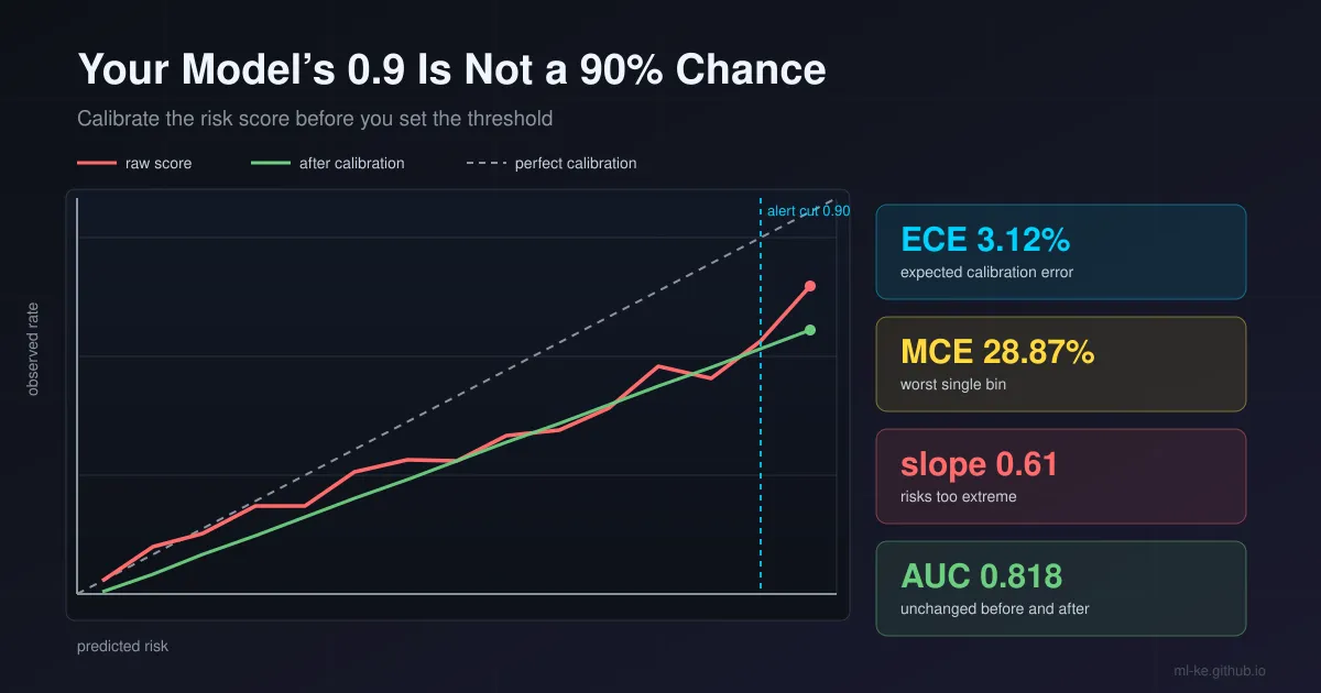
A score of 0.90 means nine out of ten, but only if the model was calibrated. Most production classifiers are not. This post builds the diagnostic, shows you the two numbers to read before ECE, and measures three fixes on a 60,000-row synthetic book.
Rank metrics have a comfortable property: they ignore the numbers. ROC-AUC and PR-AUC only care about order, so any monotone transformation of a score leaves them untouched. That is exactly why a model can pass every offline review and still waste an operations team’s week. The moment you write if score >= 0.90: escalate, you have made a claim about probability, and AUC has no opinion about whether that claim is true.
A threshold is a probability statement, in cost terms
For a single case, the cost-minimising decision is a comparison against the odds of the outcome, not against a ranking:
\[\mathbb{E}[\text{cost} \mid x] = c_{FN}\,p(x) + c_{FP}\,\bigl(1 - p(x)\bigr)\]We act when the expected cost of acting is lower than the expected cost of waiting, which makes the optimal cut a function of $p(x)$ and the two cost terms. If $p(x)$ is a ranking score wearing probability clothes, that arithmetic is fiction. The cut you picked was tuned on a validation set whose composition no longer matches production, and the queue volume moves the first time the base rate does.
Guo et al. measured how far off the numbers usually are on standard vision and NLP classifiers: most datasets and models showed some miscalibration, with ECE typically between 4% and 10%. Their CIFAR-100 ResNet-110 baseline sits at 16.53% ECE before any post-processing, a figure that falls to 1.26% with temperature scaling and to 2.66% with histogram binning. Miscalibration is not an artefact of a bad training run; it is the default state of a confident network.
Build the diagnostic before you argue about the fix
I synthesise a book of 60,000 accounts with a true event process, then a shipped score that is 1.6× sharper than reality in logit space plus noise. That is the shape models trained on rebalanced samples tend to take.
1
2
3
4
5
6
7
8
9
10
11
12
13
14
15
16
17
18
19
20
21
22
import numpy as np


def risk_data(n=60_000, seed=11):
    """A shipped risk score: trained on a rebalanced sample, so it is sharper
    than reality (temperature < 1) and systematically optimistic (+0.9 logit)."""
    rng = np.random.default_rng(seed)
    z = rng.normal(0.0, 1.0, n)
    logit_true = -2.9 + 1.4 * z
    y = (rng.random(n) < 1 / (1 + np.exp(-logit_true))).astype(int)
    logit_model = 1.6 * logit_true + 0.35 * rng.normal(0.0, 1.0, n) + 0.9
    return y, 1 / (1 + np.exp(-logit_model))


y, s = risk_data()
print(f"n = {len(y)}   observed positive rate = {y.mean() * 100:.2f}%"
      f"   mean predicted score = {s.mean() * 100:.2f}%")
print(f"{'threshold':>9} {'flagged':>8} {'share':>7} {'precision':>10}")
for t in (0.50, 0.80, 0.90):
    m = s >= t
    print(f"{t:>9.2f} {m.sum():>8d} {m.mean() * 100:>6.1f}% "
          f"{(y[m].mean() * 100 if m.any() else 0.0):>9.1f}%")
1
2
3
4
5
n = 60000   observed positive rate = 9.52%   mean predicted score = 9.62%
threshold  flagged   share  precision
     0.50     2887    4.8%      48.2%
     0.80      670    1.1%      64.5%
     0.90      269    0.4%      72.1%
The 0.90 gate is not a near-certainty gate. It flags 269 accounts, 0.4% of the book, and 72.1% of them default. The team reading that queue believes it is looking at nine-in-ten cases; it is looking at seven-in-ten cases. Everything downstream (staffing, customer communication, the cap on how many cases a reviewer can handle) was sized on the wrong number.
The reliability table is the artefact that shows where the error lives. Bin the scores, compare the mean prediction in each bin with what actually happened:
1
2
3
4
5
6
7
8
9
10
11
12
13
14
15
16
17
18
19
20
21
22
23
24
25
26
27
28
29
30
31
32
33
34
35
36
37
38
39
40
41
42
43
44
45
46
47
48
49
50
51
52
53
54
55
import numpy as np


def risk_data(n=60_000, seed=11):
    rng = np.random.default_rng(seed)
    z = rng.normal(0.0, 1.0, n)
    logit_true = -2.9 + 1.4 * z
    y = (rng.random(n) < 1 / (1 + np.exp(-logit_true))).astype(int)
    logit_model = 1.6 * logit_true + 0.35 * rng.normal(0.0, 1.0, n) + 0.9
    return y, 1 / (1 + np.exp(-logit_model))


def reliability(y, s, m=15, mode="width"):
    """Reliability table over m bins; returns rows, ECE, MCE."""
    if mode == "width":
        edges = np.linspace(0.0, 1.0, m + 1)
        idx = np.clip(np.digitize(s, edges[1:-1]), 0, m - 1)
    else:  # equal-mass: same number of scores in every bin
        order = np.argsort(s, kind="stable")
        idx = np.empty(len(s), dtype=int)
        idx[order] = np.clip(np.arange(len(s)) * m // len(s), 0, m - 1)
        edges = None
    rows, ece, mce = [], 0.0, 0.0
    for b in range(m):
        msk = idx == b
        if not msk.any():
            continue
        conf, acc = s[msk].mean(), y[msk].mean()
        gap = abs(acc - conf)
        ece += msk.mean() * gap
        mce = max(mce, gap)
        lo = edges[b] if edges is not None else float(s[msk].min())
        hi = edges[b + 1] if edges is not None else float(s[msk].max())
        rows.append((lo, hi, int(msk.sum()), conf, acc, gap))
    return rows, ece, mce


y, s = risk_data()
te = slice(len(y) // 2, len(y))
y_te, s_te = y[te], s[te]
print(f"held-out n = {len(y_te)}   positive rate = {y_te.mean() * 100:.2f}%"
      f"   mean score = {s_te.mean() * 100:.2f}%")
rows, ece, mce = reliability(y_te, s_te)
print(f"{'bin':>13} {'n':>6} {'predicted':>10} {'observed':>9} {'gap':>7}")
for lo, hi, n_b, conf, acc, gap in rows:
    print(f"{lo:.2f}-{hi:.2f} {n_b:>6d} {conf * 100:>9.1f}% {acc * 100:>8.1f}%"
          f" {gap * 100:>6.1f}%")
_, ece_mass, _ = reliability(y_te, s_te, mode="mass")
print(f"ECE (15 equal-width bins) = {ece * 100:.2f}%    MCE = {mce * 100:.2f}%")
print(f"ECE (15 equal-mass bins)  = {ece_mass * 100:.2f}%")
print(f"Brier score = {np.mean((s_te - y_te) ** 2):.4f}")
sub = np.random.default_rng(3).choice(len(y_te), 300, replace=False)
rows_sub, ece_sub, _ = reliability(y_te[sub], s_te[sub])
print(f"ECE recomputed on a 300-row spot-check sample = {ece_sub * 100:.2f}%"
      f"  (full 30,000 = {ece * 100:.2f}%)")
1
2
3
4
5
6
7
8
9
10
11
12
13
14
15
16
17
18
19
20
21
held-out n = 30000   positive rate = 9.50%   mean score = 9.62%
          bin      n  predicted  observed     gap
0.00-0.07  20538       1.6%      3.4%    1.8%
0.07-0.13   3336       9.6%     11.9%    2.2%
0.13-0.20   1630      16.4%     15.4%    1.0%
0.20-0.27   1065      23.1%     22.3%    0.8%
0.27-0.33    756      29.8%     22.2%    7.6%
0.33-0.40    610      36.4%     30.8%    5.6%
0.40-0.47    450      43.3%     34.0%    9.3%
0.47-0.53    341      49.9%     33.7%   16.2%
0.53-0.60    293      56.6%     39.9%   16.7%
0.60-0.67    237      63.2%     41.4%   21.9%
0.67-0.73    236      69.8%     47.0%   22.7%
0.73-0.80    179      76.5%     57.5%   19.0%
0.80-0.87    136      83.3%     54.4%   28.9%
0.87-0.93    125      90.1%     64.0%   26.1%
0.93-1.00     68      96.1%     77.9%   18.2%
ECE (15 equal-width bins) = 3.12%    MCE = 28.87%
ECE (15 equal-mass bins)  = 3.13%
Brier score = 0.0749
ECE recomputed on a 300-row spot-check sample = 6.35%  (full 30,000 = 3.12%)
The table has two ends, and the dangerous one is at the top: the bin that predicts 96.1% delivered 77.9%. That is the bin operators act on. The reassuring end is the summary number. An ECE of 3.12% sounds tolerable until you notice MCE, the worst single bin, at 28.87%, five times the maximum the average suggests. Mean calibration error is a weighted average, and 20,538 of 30,000 rows sit in the lowest bin where being wrong is cheap.
The last line is a warning about measurement. Recompute the same statistic on a 300-row audit sample and you get 6.35% instead of 3.12%, double the estimate from the same data. ECE is a plug-in estimator over bins, and Kumar et al. showed the popular estimators are biased with limited samples, needing roughly $O(B/\epsilon^2)$ samples for a histogram-binning estimate versus $O(1/\epsilon^2)$ for scaling methods, where $B$ is the number of distinct probabilities the model can emit. If your calibration dashboard reads from a few hundred weekly cases, it is reporting noise.
Two numbers to read before the summary statistic
The clinical prediction literature has a better vocabulary for this than the ML toolbox. Van Calster et al. define four levels of calibration: mean calibration (average predicted risk versus the event rate), weak calibration (intercept and slope), moderate calibration (the curve sits on the diagonal), and strong calibration (holds for every covariate pattern). The middle one is the cheapest to compute and the most actionable, because it splits the error into a level problem and a spread problem. Fit $\mathrm{logit}(\text{observed}) = b + a \cdot \mathrm{logit}(\text{score})$.
For reference, the calibration slope has a target of 1. A slope below 1 means the risks are too extreme: too high for the high-risk cases, too low for the low-risk ones. A slope above 1 means the risks are too timid. The intercept has a target of 0, with negative values pointing to overestimation.
1
2
3
4
5
6
7
8
9
10
11
12
13
14
15
16
17
18
19
20
21
22
23
24
25
26
27
28
29
30
31
32
33
34
35
36
37
38
39
40
41
42
43
44
45
46
47
48
49
50
51
52
53
54
55
56
57
58
59
60
61
62
63
64
65
66
67
68
69
70
71
72
73
74
75
76
77
78
79
80
81
82
83
84
85
86
87
88
89
90
91
92
93
94
95
96
97
98
99
100
101
102
103
104
105
106
107
108
109
110
111
112
113
114
115
116
117
118
119
120
121
import numpy as np


def risk_data(n=60_000, seed=11):
    rng = np.random.default_rng(seed)
    z = rng.normal(0.0, 1.0, n)
    logit_true = -2.9 + 1.4 * z
    y = (rng.random(n) < 1 / (1 + np.exp(-logit_true))).astype(int)
    logit_model = 1.6 * logit_true + 0.35 * rng.normal(0.0, 1.0, n) + 0.9
    return y, 1 / (1 + np.exp(-logit_model))


def logit(p):
    p = np.clip(p, 1e-9, 1 - 1e-9)
    return np.log(p / (1 - p))


def ece(y, p, m=15):
    edges = np.linspace(0.0, 1.0, m + 1)
    idx = np.clip(np.digitize(p, edges[1:-1]), 0, m - 1)
    return sum((idx == b).mean() * abs(y[idx == b].mean() - p[idx == b].mean())
               for b in range(m) if (idx == b).any())


def auc(y, s):
    order = np.argsort(s, kind="stable")
    ranks = np.empty(len(s), dtype=float)
    ranks[order] = np.arange(1, len(s) + 1)
    n_pos, n_neg = y.sum(), (1 - y).sum()
    return (ranks[y == 1].sum() - n_pos * (n_pos + 1) / 2) / (n_pos * n_neg)


def fit_logistic(y, X, iters=60):
    """Newton/IRLS for logit(observed) = X @ w. Returns the coefficient vector."""
    k = X.shape[1]
    w = np.zeros(k)
    for _ in range(iters):
        p = 1 / (1 + np.exp(-X @ w))
        wd = p * (1 - p)
        step = np.linalg.solve(X.T @ (X * wd[:, None]) + 1e-9 * np.eye(k), X.T @ (y - p))
        w = w + step
        if np.max(np.abs(step)) < 1e-11:
            break
    return w


def fit_temperature(y, z, lo=0.2, hi=5.0, iters=160):
    """One-parameter temperature scaling, golden-section search on NLL."""
    phi = (5 ** 0.5 - 1) / 2

    def nll(T):
        p = np.clip(1 / (1 + np.exp(-z / T)), 1e-12, 1 - 1e-12)
        return -np.mean(y * np.log(p) + (1 - y) * np.log(1 - p))

    x1, x2 = hi - phi * (hi - lo), lo + phi * (hi - lo)
    f1, f2 = nll(x1), nll(x2)
    for _ in range(iters):
        if f1 < f2:
            hi, x2, f2 = x2, x1, f1
            x1 = hi - phi * (hi - lo)
            f1 = nll(x1)
        else:
            lo, x1, f1 = x1, x2, f2
            x2 = lo + phi * (hi - lo)
            f2 = nll(x2)
    return (lo + hi) / 2


def murphy(y, p, nd=2):
    """Brier = reliability - resolution + uncertainty, grouped by 2-dp score."""
    q = np.round(p, nd)
    base = y.mean()
    rel = res = 0.0
    for v in np.unique(q):
        msk = q == v
        rel += msk.mean() * (v - y[msk].mean()) ** 2
        res += msk.mean() * (y[msk].mean() - base) ** 2
    return rel, res, base * (1 - base)


y, s = risk_data()
cal, te = slice(0, len(y) // 2), slice(len(y) // 2, len(y))
y_c, s_c = y[cal], s[cal]
y_te, s_te = y[te], s[te]
z_te, base = logit(s_te), y_te.mean()

b_a, a_a = fit_logistic(y_c, np.column_stack([np.ones_like(s_c), logit(s_c)]))

# Intercept-only recalibration: logit(p) = logit(score) + c, slope pinned at 1.
c = 0.0
for _ in range(60):
    p_tmp = 1 / (1 + np.exp(-(logit(s_c) + c)))
    step = (y_c - p_tmp).sum() / (p_tmp * (1 - p_tmp)).sum()
    c += step
    if abs(step) < 1e-12:
        break
p_shift = 1 / (1 + np.exp(-(logit(s_te) + c)))

T = fit_temperature(y_c, logit(s_c))
p_temp = 1 / (1 + np.exp(-z_te / T))
p_platt = 1 / (1 + np.exp(-(b_a + a_a * z_te)))

print(f"weak calibration: intercept b = {b_a:+.3f} (target 0), slope a = {a_a:.3f} "
      f"(target 1); level shift c = {c:+.3f}; T = {T:.3f}")
print(f"{'variant':>22} {'ECE':>8} {'Brier':>8} {'level':>9} {'flagged@0.90':>13}")
for name, p in [("raw score", s_te), (f"logit shift {c:+.2f}", p_shift),
                (f"temperature T={T:.3f}", p_temp),
                (f"Platt b={b_a:+.2f} a={a_a:.3f}", p_platt)]:
    print(f"{name:>22} {ece(y_te, p) * 100:>7.2f}% "
          f"{np.mean((p - y_te) ** 2):>8.4f} {(p.mean() - base) * 100:>+8.2f} "
          f"{(p >= 0.90).sum():>12d}")
print(f"ROC-AUC raw = {auc(y_te, s_te):.4f}   Platt = {auc(y_te, p_platt):.4f} "
      f"(unchanged: both fits are monotone)")
m = s_te >= 0.90
print(f"the {m.sum()} accounts above the raw 0.90 cut: raw score >= 0.90, "
      f"calibrated {p_platt[m].min():.2f}-{p_platt[m].max():.2f} "
      f"(mean {p_platt[m].mean():.2f}); they actually defaulted "
      f"{y_te[m].mean() * 100:.1f}% of the time")
rel, res, unc = murphy(y_te, p_platt)
print(f"Brier = reliability {rel:.4f} - resolution {res:.4f} + uncertainty {unc:.4f}"
      f" = {rel - res + unc:.4f}   (direct {np.mean((p_platt - y_te) ** 2):.4f})")
1
2
3
4
5
6
7
8
9
weak calibration: intercept b = -0.626 (target 0), slope a = 0.613 (target 1); level shift c = -0.015; T = 1.259
               variant      ECE    Brier     level  flagged@0.90
             raw score    3.12%   0.0749    +0.12          135
     logit shift -0.01    3.11%   0.0748    +0.03          134
   temperature T=1.259    2.69%   0.0747    +2.28           58
 Platt b=-0.63 a=0.613    0.34%   0.0720    +0.01            4
ROC-AUC raw = 0.8179   Platt = 0.8179 (unchanged: both fits are monotone)
the 135 accounts above the raw 0.90 cut: raw score >= 0.90, calibrated 0.67-0.95 (mean 0.75); they actually defaulted 69.6% of the time
Brier = reliability 0.0005 - resolution 0.0145 + uncertainty 0.0860 = 0.0720   (direct 0.0720)
A logit shift does nothing when the level is already right. Fitting only an intercept moved the mean from 9.62% to 9.53%, a shift of −0.015 logits, with ECE at 3.11% and the queue going from 135 to 134. This is worth internalising because the opposite case is common: van den Goorbergh et al. simulated logistic risk models across event fractions and found that training on imbalance-corrected data produced median calibration intercepts of −4.5 or lower at a 1% event fraction, meaning severe systematic overestimation of the minority-class probability. Adding an intercept-only recalibration step brought those back to between −0.07 and 0.03. If your score was trained on SMOTE’d or class-weighted data, expect a level error and fix the level. Do not expect a level fix to repair a spread error.
Temperature scaling is one knob, and the book needed two. The single-parameter version improved ECE from 3.12% to 2.69%, about 14% lower in relative terms, while pushing the average prediction from +0.12 to +2.28 points above the observed rate. ECE improved and calibration-in-the-large got worse. That is not a contradiction; it is what happens when you optimise one scalar against a two-dimensional problem. Guo et al. found temperature scaling “surprisingly effective” on image and document classifiers because their error was mostly spread. Here the error had both components, so one parameter could only trade one for the other.
Platt scaling carries both, and the ranking survives. Fitting intercept and slope together gives $b = -0.63$, $a = 0.613$, ECE 0.34%, level +0.01 points, and a Brier score down from 0.0749 to 0.0720. ROC-AUC is 0.8179 before and after, identical, because a strictly monotone map cannot reorder anything. You lose no discrimination by calibrating; you only change what the numbers mean. That matters for the deployment conversation: nobody has to defend a new model version, because the scores map one-to-one onto the old ones.
What the fix actually changes for the queue
The operational payoff is not the ECE line. It is the accounts the cut selects. All 135 rows above the raw 0.90 cut on the held-out half carry calibrated probabilities between 0.67 and 0.95, with a mean of 0.75, and they defaulted 69.6% of the time. The threshold was never measuring what the runbook said it measured. After calibration, a 0.90 cut flags 4 accounts out of 30,000, because a genuine 90% default risk is rare in this book.
That leaves a decision rather than an algorithm: either lower the cut and accept a larger queue of lower-confidence cases, or keep the exclusivity of the current queue and stop describing it as near-certain. Pick the cut from the cost ratio and the reviewer capacity, then read the calibrated probability as an expected loss rate per case, the only form in which the number survives contact with a finance team.
The decomposition: is the score informative, or just wrong?
Murphy’s 1973 partition splits the Brier score into three parts, and the split separates a modelling failure from a measurement ceiling:
\[\mathrm{BS} = \mathrm{REL} - \mathrm{RES} + \mathrm{UNC}\]On the calibrated held-out scores: reliability 0.0005, resolution 0.0145, uncertainty 0.0860, summing to 0.0720 and matching the direct Brier calculation to four decimals.
Reliability is the part calibration can remove. Resolution is the part your features bought: the score separates 9.50%-base-rate outcomes into groups whose rates span a wide range, and that span is worth 0.0145. Uncertainty is arithmetic. With a 9.50% base rate, guessing the base rate every time already costs 0.0860, and no model can reduce it. A useful consequence: if a model review reports “calibration is fine, we just need better features”, the decomposition says which term is actually large. Ours was dominated by uncertainty, which is another way of saying the ceiling in this problem is not a bug in the score.
Where teams get this wrong
- Fitting the calibrator on training rows. The calibration map then inherits the model’s optimism and pushes probabilities further from 0.5 than they should be. Use a held-out split disjoint from training; scikit-learn’s
CalibratedClassifierCVbuilds that split through cross-validation for you. - Reading a summary statistic off a small sample. As the 300-row recompute showed, ECE moved from 3.12% to 6.35% on the same model. Fix the binning scheme, log the sample size beside the number, and treat small-sample ECE as indicative only.
- Shipping isotonic regression on thin data. Isotonic is more flexible — it can correct any monotonic distortion — but scikit-learn’s guidance is that it overfits on small datasets and only reliably matches sigmoid once you have more than roughly 1,000 samples. Isotonic also produces ties in the output, so it can change ROC-AUC, while sigmoid keeps the ranking intact.
- Using class weighting or resampling as the whole fix. The simulated evidence is blunt: imbalance correction did not improve AUROC, and it created large negative calibration intercepts that only recalibration repaired.
- Treating one threshold as universal. Calibration is a property of a model and a population. Refit on recent data, and check the reliability table per segment before assuming a national threshold holds in one county.
How to apply it
| Step | Concrete check |
|---|---|
| Split honestly | Calibrator fit on rows disjoint from training; prefer cross-validated folds |
| Size the sample | 1,000+ rows for a curve; the clinical rule of thumb is 200 events and 200 non-events for a stable curve |
| Fit level and slope | logit(y) = b + a·logit(score); report $b$, $a$, and the event rate beside them |
| Choose the fix by the diagnosis | Level error → intercept shift (or the imbalance-corrected case); spread error → temperature or Platt; both → Platt |
| Re-check the queue | Report flagged volume and precision at the production cut, before and after |
| Keep rank metrics separate | AUC/PR-AUC as the discrimination check; never as the calibration check |
| Monitor drift | ECE and the reliability table on a rolling window, with a stated sample-size floor |
A sequencing that survives a release process: run the reliability table and the intercept/slope fit as a notebook gate before promotion, store the fitted map next to the model artefact so served probabilities are reproducible, then recompute a rolling ECE in monitoring on a fixed binning scheme. When only the level drifts, which is a common pattern after the base rate moves, an intercept-only refit is enough and cheap to automate. When the slope drifts, the score itself has gone stale and retraining is the honest fix. Recalibration sharpens a ranking; it cannot create signal that the features never carried.
Key takeaways
| Takeaway | Evidence in this post |
|---|---|
| A great AUC does not make a score a probability | ROC-AUC 0.8179 unchanged by calibration; the 0.90 cut’s precision was 72.1% raw |
| Read the worst bin, not just the average | ECE 3.12% against MCE 28.87%; the 0.93–1.00 bin predicted 96.1% and delivered 77.9% |
| Split the error into level and slope before choosing a fix | Intercept −0.626, slope 0.613; an intercept-only shift changed ECE by 0.01 points |
| One parameter can trade ECE against the average | Temperature scaling improved ECE to 2.69% while the level moved to +2.28 points |
| Two parameters fixed both, at no cost in ranking | ECE 0.34%, level +0.01 points, Brier 0.0749 → 0.0720, AUC identical |
| Calibration is not a substitute for signal | Reliability 0.0005 versus resolution 0.0145 and uncertainty 0.0860 |
The demo is synthetic, with 60,000 rows and a seeded generator so every number above reproduces. The procedure transfers directly to a credit, claims, churn, or fraud score: same two diagnostics, same two fixes, and a queue whose size you can finally explain.
References
- Guo, C., Pleiss, G., Sun, Y., Weinberger, K. Q. (2017). On Calibration of Modern Neural Networks — ICML 2017; ECE definition, temperature scaling, Table 1 ECE figures.
- Kumar, A., Liang, P., Ma, T. (2019). Verified Uncertainty Calibration — NeurIPS 2019 spotlight; bias in plug-in ECE estimators, sample-complexity comparison.
- Van Calster, B., McLernon, D. J., van Smeden, M., Wynants, L., Steyerberg, E. W. (2019). Calibration: the Achilles heel of predictive analytics — BMC Medicine 17, 230; mean, weak, moderate and strong calibration.
- Van Calster, B., Nieboer, D., Vergouwe, Y., De Cock, B., Pencina, M. J., Steyerberg, E. W. (2016). A calibration hierarchy for risk models was defined — Journal of Clinical Epidemiology 74, 167–176.
- van den Goorbergh, R., van Smeden, M., Timmerman, D., Van Calster, B. (2022). The harm of class imbalance corrections for risk prediction models — JAMIA 29(9), 1525–1531.
- Murphy, A. H. (1973). A New Vector Partition of the Probability Score — Journal of Applied Meteorology 12(4), 595–600.
- scikit-learn developers. Probability calibration — sigmoid versus isotonic behaviour, sample-size guidance, and the effect on ranking metrics.
Related posts
- The Denominator Is the Metric: Auditing a RAG Retriever Before You Blame the Model — measuring retrieval before blaming the generator.
- Fraud Models Rot Quietly: PSI, Feature Drift and Data-Quality Gates in Production — the monitoring layer that catches a score going stale.
- Split Before You Believe: Why Offline Fraud Models Score Better Than They Perform — the validation split that decides whether these numbers are even testable.
- Thirty Times Smaller: Auditing Embedding Compression Before You Ship It — the same audit-before-you-ship discipline, applied to vectors.