Words In, Enzymes Out: What Two Protein-Design Releases Actually Delivered
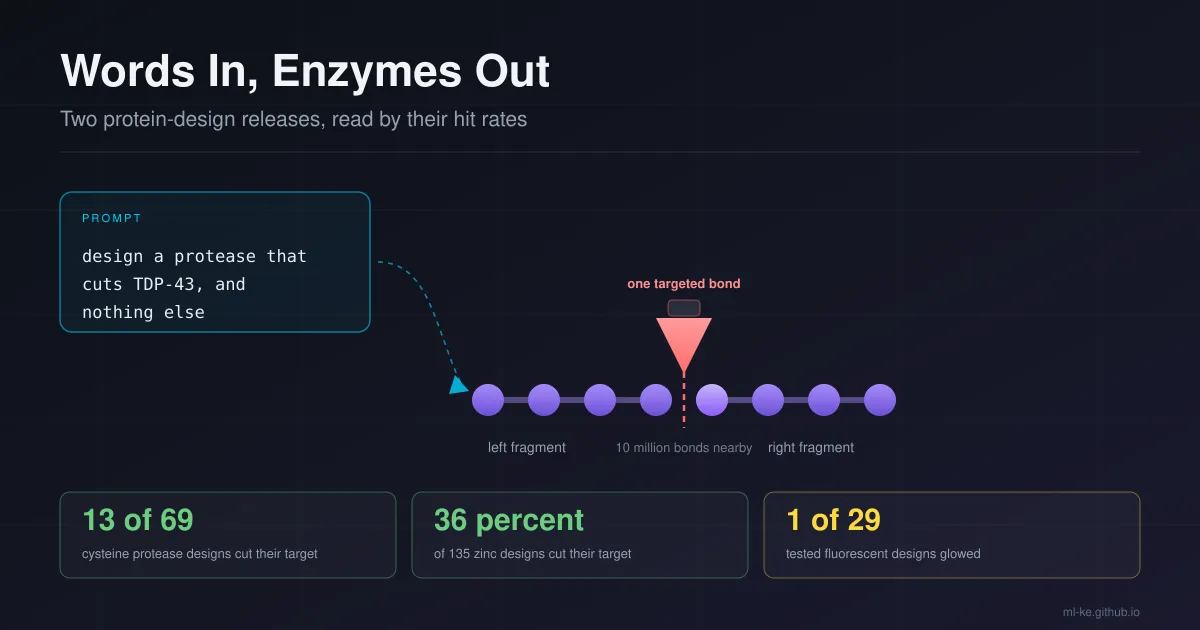
In one paragraph: In October and November 2026, two groups published protein design results that crossed the same line from different directions. At Westlake University, a 16-billion-parameter model called Pinal took plain-language descriptions of a job and returned candidate proteins, and four of four design tasks produced the intended function in the lab. At the University of Washington’s Institute for Protein Design, RFdiffusion variants produced de novo proteases, enzymes that cut chosen proteins, including full-length TDP-43, which aggregates in ALS. Both releases published their hit rates, which is what makes them worth reading carefully: 19 percent of 69 cysteine protease designs worked, 36 percent of 135 zinc designs worked, and one of 29 tested fluorescent-protein designs glowed. The headline is that AI designs proteins. The number that changes what you do next is the rate, and what its denominator was.
This blog has covered the computational biology stack from the data end: variant-effect maps from a genome model and a pangenome release that gives breeders something to select on. It has also covered what happens when a model reaches a clinic or a field, where the deployment record is the evidence. This is the first post here on de novo design of function, and the reason to write it now is narrow. Design papers used to report a handful of successes and leave the denominator implicit. These two report the denominator, in public, in the abstract, which means the results can be planned against rather than admired.
What shipped in one month
Two different methods, one shared premise: write the function down first, then build a protein around it, instead of taking a natural protein and optimizing it.
| Pinal | De novo proteases | |
|---|---|---|
| Group | Westlake University, China | Institute for Protein Design, University of Washington |
| Published | Nature, 2026, DOI 10.1038/s41586-026-11205-z | Two Nature papers, 14 October 2026, DOI 10.1038/s41586-026-11167-2 and 10.1038/s41586-026-11143-w |
| Method | A 16B-parameter foundation model over protein-text pairs | RFdiffusion, in a variant specialised for enzyme design and protein-protein interfaces |
| Input | A sentence describing the function | A target epitope, plus a catalytic mechanism to install |
| Training or design basis | 1.7 billion synthetically annotated protein-text pairs, built from 135 million sequences; predicted structures from an AlphaFold database | Diffusion over backbone geometry; the catalytic core of a natural protease is kept and everything around it is designed |
| Lab validation | Four tasks: fluorescent protein, PET hydrolase, alcohol dehydrogenase, metabolic H-protein | Amide-bond cleavage of designed peptide substrates; then full-length proteins |
| Published hit rate | 1 of 29 fluorescent designs; 5 of 20 H-protein designs | 13 of 69 cysteine protease designs (19 percent); 36 percent of 135 zinc designs |
| Availability | Behind a subscription paywall at the time of writing; no open-weights statement in the abstract | Methods build on the released RFdiffusion code |
Pinal’s two modules are worth naming because they explain the interface. The first, T2struct, turns the sentence into a one-dimensional structural blueprint. The second, SaProt-T, reads that blueprint together with the original text and emits an amino acid sequence. The model generates several blueprints, designs a sequence for each, scores the pairs, and returns the best. Training data came from 135 million protein sequences whose functions were described in plain language by other models and existing annotations, giving 1.7 billion pairs, with three-dimensional structures pulled from an AlphaFold database rather than solved in a lab.
The protease work starts from the opposite end. A protease’s catalytic centre is a handful of amino acids in tight proximity with a supporting scaffold that holds them at the right angles. The Institute for Protein Design team kept the catalytic core of two natural mechanisms, a zinc metalloprotease and a cysteine protease, and had RFdiffusion design the rest of the protein: the pocket that binds the target sequence, and the scaffold that positions the catalytic residues against the bond to be cut. Ars Technica described it as short-circuiting the diversification process, replacing the entire rest of the protein rather than mutating it.
The text interface matters because of what it replaces. The Pinal abstract is explicit about the two limits of earlier design models: they need a natural protein as a starting point to optimise, or they need the user to reformulate a functional goal as geometric and sequence-level constraints that guide generation. Both routes require the person writing the prompt to already know the answer’s shape. A sentence like “design a plastic-degrading enzyme” removes that requirement, and it is why the same model can be pointed at a fluorescent protein, a PET hydrolase, an alcohol dehydrogenase and a metabolic H-protein without a new pipeline for each.
Two of those four tasks are environmental rather than medical, which is the part of this release that gets least attention. A PET hydrolase breaks down polyethylene terephthalate, the plastic in drink bottles. An H-protein is a shuttle in a multi-enzyme pathway that fixes carbon dioxide. A design method that can be asked for either is a design method aimed at industrial and climate problems, not only at drugs.
What came out is not a new chemistry. It is a known mechanism installed in a designed pocket, which is a smaller claim than “AI invented an enzyme” and a more useful one, because the design problem becomes the specificity of the pocket rather than the reactivity of the site.
Reading the hit rate instead of the headline
Four numbers came out of these papers, and they are not comparable at face value because the denominators differ. Put intervals on them and the picture changes again.
1
2
3
4
5
6
7
8
9
10
11
12
13
14
15
16
17
18
19
20
21
22
23
24
25
import math

def wilson(k, n, z=1.96):
    p = k / n
    denom = 1 + z * z / n
    centre = (p + z * z / (2 * n)) / denom
    half = z * math.sqrt(p * (1 - p) / n + z * z / (4 * n * n)) / denom
    return p, max(0.0, centre - half), min(1.0, centre + half)

runs = [
    ("cysteine proteases", 13, 69),
    ("zinc metalloproteases", round(0.36 * 135), 135),
    ("fluorescent protein (Pinal)", 1, 29),
    ("metabolic H-protein (Pinal)", 5, 20),
]

print(f"{'design task':30s} {'worked':>7s} {'tested':>7s} {'rate':>7s}  95% interval")
for name, k, n in runs:
    p, lo, hi = wilson(k, n)
    print(f"{name:30s} {k:>7d} {n:>7d} {p:>7.3f}  [{lo:.3f}, {hi:.3f}]")

p1, lo1, hi1 = wilson(13, 69)
p2, lo2, hi2 = wilson(1, 29)
print(f"\ncysteine lower bound {lo1:.3f} vs fluorescent upper bound {hi2:.3f}")
print(f"intervals overlap: {lo1 < hi2}")
1
2
3
4
5
6
7
8
design task                     worked  tested    rate  95% interval
cysteine proteases                  13      69   0.188  [0.114, 0.296]
zinc metalloproteases               49     135   0.363  [0.287, 0.447]
fluorescent protein (Pinal)          1      29   0.034  [0.006, 0.172]
metabolic H-protein (Pinal)          5      20   0.250  [0.112, 0.469]

cysteine lower bound 0.114 vs fluorescent upper bound 0.172
intervals overlap: True
The overlap at the bottom is the point. A 19 percent success rate measured on 69 designs and a 3.4 percent rate measured on 29 designs cannot be told apart: the cysteine interval starts at 0.114, the fluorescent interval ends at 0.172, so a single 29-design batch is consistent with anything from a hopeless model to a good one. The 36 percent zinc figure is tighter only because 135 designs were tested, not because the method is a different category.
Then there is the denominator that does not appear in the headline at all. The fluorescent protein task generated 50,000 sequences, filtered them to 29 for synthesis and assay, and one worked. The 3.4 percent describes the shortlist. It says nothing about the model’s raw output, because 49,971 designs were never tested, and it says nothing about an unfiltered pipeline. Two rates hide in that one sentence, and a reader who quotes 1-in-29 as the model’s success rate is quoting the wrong population.
This is the same failure mode as reading a screening tool’s aggregate accuracy without asking what prevalence it was measured at, or reading a benchmark score without checking for contamination. The number is real. The question is what it is a rate over.
The filter is the product
If you take the generation-to-assay funnel seriously, the ranking step becomes the most valuable thing in the release, and its value is measurable.
1
2
3
4
5
6
7
8
9
10
11
12
13
14
15
16
17
18
19
20
21
22
23
import math

GENERATED = 50_000
TESTED = 29
ASSAY_COST = 80.0          # assumed: synthesis plus one assay per construct, USD

print(f"generated {GENERATED:,} designs, tested {TESTED}")
print(f"share of the batch assayed: {100 * TESTED / GENERATED:.3f}%")
print(f"cost of the ranked shortlist: ${TESTED * ASSAY_COST:,.0f}")
print(f"cost of assaying the whole batch: ${GENERATED * ASSAY_COST:,.0f}")
print(f"ratio: {GENERATED / TESTED:,.0f}x")

def tests_for_one_hit(p, conf=0.90):
    return math.ceil(math.log(1 - conf) / math.log(1 - p))

print()
for label, k, n in [("fluorescent protein", 1, 29),
                    ("metabolic H-protein", 5, 20),
                    ("cysteine protease", 13, 69),
                    ("zinc metalloprotease", round(0.36 * 135), 135)]:
    p = k / n
    print(f"{label:22s} rate {p:.3f}  tests for 90% chance of one hit {tests_for_one_hit(p):>3d}"
          f"  expected tests for five hits {math.ceil(5 / p):>4d}")
1
2
3
4
5
6
7
8
9
10
generated 50,000 designs, tested 29
share of the batch assayed: 0.058%
cost of the ranked shortlist: $2,320
cost of assaying the whole batch: $4,000,000
ratio: 1,724x

fluorescent protein    rate 0.034  tests for 90% chance of one hit  66  expected tests for five hits  145
metabolic H-protein    rate 0.250  tests for 90% chance of one hit   9  expected tests for five hits   20
cysteine protease      rate 0.188  tests for 90% chance of one hit  12  expected tests for five hits   27
zinc metalloprotease   rate 0.363  tests for 90% chance of one hit   6  expected tests for five hits   14
The $4,000,000 figure is a model, not a measurement: it takes an assumed $80 per synthesised and assayed construct and applies it to all 50,000 designs. The assumption is labelled so you can replace it with your own number. What survives a change in the assumption is the ratio, 1,724 to 1, which is the model’s ranking contribution expressed as the cost it avoids. At 3.4 percent you need to test about 66 designs to have a 90 percent chance of one working protein, and about 145 to expect five. At 36 percent the same two figures are 6 and 14.
That last table is the practical output of the whole release, and it is a table you can build for your own pipeline as soon as you have one number: the hit rate on your own assays, with its denominator. A lab that knows it needs five working designs can size the batch, and a lab that only knows a headline rate cannot.
There is a second reading of the same arithmetic, and it is less flattering. If your filter selects well but your generator produces mostly non-functional proteins, the funnel works and the synthesis bill stays small. If your filter is weak, you test hundreds of designs and the same rate costs an order of magnitude more. The published numbers cannot separate a model that generates good candidates from a scoring function that ranks mediocre ones well, because both produce the same shortlist.
What the abstract says about the ranking signal is worth quoting for that reason: candidates combined high predicted foldability with functional-description alignment and sequence diversity. Three separate scores, and only the first two are about the design working. The diversity term exists because a shortlist of 29 near-identical sequences tests one hypothesis 29 times. When you audit a design pipeline, those three terms are where the sensitivity sits: a filter that over-weights foldability returns well-folded proteins that do nothing, and a filter without a diversity term returns the same protein 29 times.
The interval from the hit-rate section also has a budget consequence, and it is larger than the point estimate suggests.
1
2
3
4
5
6
7
8
9
10
11
12
13
14
15
16
17
18
19
20
21
22
import math

ASSAY_COST = 80.0

def wilson(k, n, z=1.96):
    p = k / n
    denom = 1 + z * z / n
    centre = (p + z * z / (2 * n)) / denom
    half = z * math.sqrt(p * (1 - p) / n + z * z / (4 * n * n)) / denom
    return max(0.0, centre - half), min(1.0, centre + half)

def assays_for(p, conf=0.90):
    return math.ceil(math.log(1 - conf) / math.log(1 - p))

for label, k, n in [("fluorescent protein", 1, 29), ("metabolic H-protein", 5, 20)]:
    lo, hi = wilson(k, n)
    n_lo, n_hi = assays_for(lo), assays_for(hi)
    print(f"{label}, observed {k}/{n}: true rate in [{lo:.3f}, {hi:.3f}]")
    print(f"  assays for a 90% chance of one working design: {n_lo} at the low end, {n_hi} at the high end")
    print(f"  budget at ${ASSAY_COST:.0f} per assay: ${n_lo * ASSAY_COST:,.0f} to ${n_hi * ASSAY_COST:,.0f}")
    print(f"  spread: {n_lo / n_hi:.1f}x")
    print()
1
2
3
4
5
6
7
8
9
fluorescent protein, observed 1/29: true rate in [0.006, 0.172]
  assays for a 90% chance of one working design: 376 at the low end, 13 at the high end
  budget at $80 per assay: $30,080 to $1,040
  spread: 28.9x

metabolic H-protein, observed 5/20: true rate in [0.112, 0.469]
  assays for a 90% chance of one working design: 20 at the low end, 4 at the high end
  budget at $80 per assay: $1,600 to $320
  spread: 5.0x
A single 29-design experiment that produced one hit is consistent with a first campaign cost of $1,040 or $30,080, and the paper cannot tell you which. The H-protein task, with 5 of 20, narrows to a factor of five. This is the argument for reporting intervals rather than rates: the interval is what a budget can be built on, and the point estimate is a number that hides the decision.
Why the cut has to be specific
The proteases make the specificity problem concrete, and it is where a protein design result can go wrong in a way an image model cannot. A peptide bond in water has a half-life of several hundred years without an enzyme. Evolution solved that with a small number of catalytic mechanisms, and every one of them is fast enough that the limiting factor is not speed but where the enzyme cuts.
The arithmetic of that constraint uses the size of the human proteome against the size of the recognition site.
1
2
3
4
5
6
7
8
9
10
11
12
13
14
15
16
17
PROTEINS = 20_000      # approximate count of reviewed human proteins
MEAN_LEN = 500         # approximate mean length, residues
FREQ_CYS = 0.023       # cysteine share of residues in the human proteome

def windows(k):
    return PROTEINS * (MEAN_LEN - k + 1)

print(f"{'site length':>11s} {'chance matches in the human proteome':>38s}")
for k in (3, 4, 5, 6, 7, 8):
    print(f"{k:>11d} {windows(k) / 20 ** k:>38.3f}")

k = 6
uniform = windows(k) / 20 ** k
one_cys = windows(k) * FREQ_CYS * (1 / 20) ** (k - 1)
print(f"\n6-residue site, any composition:      {uniform:.3f} expected off-target windows")
print(f"6-residue site, cysteine at position 1: {one_cys:.3f}")
print(f"gain from one rare residue: {uniform / one_cys:.2f}x")
1
2
3
4
5
6
7
8
9
10
11
site length   chance matches in the human proteome
          3                               1245.000
          4                                 62.125
          5                                  3.100
          6                                  0.155
          7                                  0.008
          8                                  0.000

6-residue site, any composition:      0.155 expected off-target windows
6-residue site, cysteine at position 1: 0.071
gain from one rare residue: 2.17x
A three-residue recognition rule matches about 1,245 places in the proteome by chance. Four residues, 62. Five residues, 3. The number only falls below one at six residues, and below 0.01 at seven. Those are chance matches under a uniform residue distribution, so they are a floor rather than an estimate: real sites are more structured, and a residue that is rarer than average buys you a factor of two, not a factor of a hundred.
The floor is also pessimistic in one direction, because a designed pocket does not read a protein one-dimensionally. Fold a chain and residues that sit far apart in sequence end up adjacent in space, so a protease can contact a surface of eight or ten residues drawn from three separate loops. That is how natural proteases manage to be selective, and it is what a designed pocket has to reproduce. The linear-window arithmetic above tells you the minimum information a site needs; the three-dimensional contacts are how a design gets past that minimum.
This is why the papers report cleavage of cognate peptide substrates first. A designed peptide of the right sequence is the easy test. Cutting a full-length cellular protein at one bond while leaving the other ~10 million peptide bonds alone is the same problem one level up, and it is the result that matters therapeutically. The team’s own summary of the cysteine work is that de novo enzyme design has advanced well beyond model reactions on activated substrates, which is a fair reading of 19 percent on a real amide bond.
It also explains why the report of a cysteine protease that cut at precisely the intended site is the most interesting line in the coverage. Precision at the scissile bond is the property that separates a research reagent from something you would put in a cell. The proteases have not been in human trials, and off-target proteolysis is exactly the kind of failure a trial would have to rule out.
What the results do and do not support
| Claim | What the sources support |
|---|---|
| A language model designed proteins from text alone | Pinal’s abstract: candidate proteins generated from natural-language descriptions of desired function, four tasks, intended function observed in each |
| The designs worked without further optimisation | The H-protein result was obtained without iterative experimental optimisation, and raised product titre 1.7-fold over the native E. coli H-protein |
| Design success is now predictable enough to plan around | 13/69 and 36 percent of 135 for proteases; 5/20 for the H-protein; 1/29 for the fluorescent protein |
| AI designed entirely new enzymes | Partly: the catalytic cores come from natural zinc and cysteine proteases, and the surrounding scaffold and pocket are designed |
| The designed proteases are therapeutic candidates | Not yet: they cleaved TDP-43, amyloid-beta fragments and serum amyloid A in the lab, and have not been tested in humans |
| The fluorescent protein result was strong | Weakest of the four: 50,000 generated, 29 tested, one glowed, and the authors say precise emission-wavelength control is still hard |
| Computational scores stand in for assays | They do not: the abstract reports high predicted foldability and functional alignment, which is a prioritisation signal, and the experimental numbers are the evidence |
The honest summary of the Pinal release is that the interface works and the reliability is uneven. Four of four tasks produced the intended function, which is a better record than most design papers manage, and two of those four were enzymes with measurable catalytic activity. Against that, the fluorescent protein task needed 50,000 generated designs to yield one working sequence from 29 tested, and the model could not be steered to a specific emission wavelength. A model that can be asked for “a fluorescent protein” but not “a green one” is a candidate generator, not a specification language.
The honest summary of the protease release is that a known mechanism now has a designable pocket. A 36 percent hit rate on a zinc site is high enough that a lab can plan a campaign around it, and the 30-fold gain in cutting speed after AI-guided refinement shows the second round of design is where a lot of the performance comes from. Note what that gain is: kinetics on designs that already worked, not a higher share of designs that work. What the release does not show is that arbitrary targets are equally tractable. The successful targets were chosen because a peptide sequence and a binding pocket could be specified, and that is not true of every protein you might want to cleave.
How to apply this
If you are on the wet-lab side, the order below keeps a design campaign honest from the first batch.
- Record the denominator before you record the rate. Differentiate designs generated from designs synthesised from designs assayed. The 1-in-29 figure in the Pinal release is a rate over a filtered shortlist, and quoting it as the model’s success rate overstates nothing except your confidence.
- Plan batch size from a rate you measured yourself. Sixty-six assays for a 90 percent chance of one hit at 3.4 percent, six at 36 percent. Replace both numbers with your own, then size the batch.
- Budget a second round for kinetics, not for hits. The 30-fold gain after refinement was cutting speed on designs that had already cleared the assay. A first-round design that cuts slowly is still a candidate worth refining, and a plan that stops at round one has no route to it.
- Treat recognition-site length as the specificity specification. A four-residue rule has 62 chance matches in the human proteome. If you cannot get to six or seven, the assay that matters is the off-target one, not the on-target one.
- Test the shortlist against the hardest substrate you have. A cognate peptide is the easy test. The full-length protein, in the presence of other proteins, is the result that travels.
If you are building models rather than proteins, two things transfer.
- Publish the funnel, not the demo. Every design system has a generation count, a filter, and an assay count. The three numbers together are the result; any one alone is marketing.
- Report intervals at small n. Twenty-nine assays gave a budget range of $1,040 to $30,080 for a 90 percent chance of one working design. That is not a criticism of the paper, it is the arithmetic of small samples, and the interval belongs next to the point estimate wherever a number will be used to size a programme.
For a funder or a research group in a low-resource setting, the useful part of these releases is not the parameter count. It is that the expensive step moved. Pinal’s generation is the part that needs a GPU; the assay is the part that needs a wet lab, and a 36 percent hit rate means the wet-lab bill for a first campaign is small enough to plan. A group that can run 96 assays and read the output of a structural model can now compete on target choice rather than on compute, provided it has a scoring function it trusts.
Key takeaways
| Claim | What the sources support |
|---|---|
| Two independent groups crossed into functional de novo design within a month | Pinal in Nature, protease papers on 14 October 2026, both body-verified |
| The most useful number in each release is the hit rate | 13/69 (19 percent), 36 percent of 135, 5/20, 1/29 |
| A 29-design batch cannot distinguish a good model from a mediocre one | Cysteine interval [0.114, 0.296] overlaps fluorescent interval [0.006, 0.172] |
| The published fluorescent rate is a rate over a filtered shortlist | 50,000 generated, 29 tested, one worked: 0.058 percent of the batch was assayed |
| Planning needs about 66 assays for one hit at 3.4 percent | And 6 at 36 percent, 9 at 25 percent, 12 at 19 percent |
| Specificity is set by recognition-site length, not catalytic chemistry | A 4-residue rule has 62 chance matches in an approximate human proteome; a 6-residue rule has 0.16 |
| The designed proteases are a platform, not a drug | Cleaved TDP-43, amyloid-beta fragments and serum amyloid A in the lab; no human trials |
| The catalytic chemistry is borrowed, the pocket is designed | Zinc and cysteine catalytic cores retained; scaffold and substrate pocket designed by RFdiffusion |
| A second design round carries much of the kinetics | 30-fold faster cutting after AI-guided refinement of the best zinc designs |
References
- Anqi Chen et al., Computational design of metalloproteases, Nature, 14 October 2026 — https://www.nature.com/articles/s41586-026-11167-2
- Hojae Choi et al., De novo design of cysteine proteases, Nature, 14 October 2026 — https://www.nature.com/articles/s41586-026-11143-w
- Fengyuan Dai et al., Programmable design of functional proteins from natural language, Nature, 2026 — https://www.nature.com/articles/s41586-026-11205-z
- Phys.org, AI designs working molecular scissors that recognize and cut selected protein targets (16 October 2026) — https://phys.org/news/2026-10-ai-molecular-scissors-protein.html
- Phys.org, Tell this AI what you want a protein to do, and it designs one (November 2026) — https://phys.org/news/2026-11-ai-protein.html
- Chemical and Engineering News, Researchers use AI to design protein-digesting enzymes (20 October 2026) — https://cen.acs.org/physical-chemistry/protein-folding/ai-design-protein-protease/104/web/2026/10
- Ars Technica, Researchers use AI to design proteins that cut up other proteins (14 October 2026) — https://arstechnica.com/science/2026/10/researchers-use-ai-to-design-proteins-that-cut-up-other-proteins/
Related posts
- Nine Billion Variants, One Atlas: What DeepMind’s AlphaGenome Atlas Makes Testable — the prediction side of computational biology, and what a precomputed effect table is good for.
- Is Your +3-Point Eval Gain Real? Gating a Comparison with Paired Statistics — the small-sample statistics behind the intervals in this post.
- 44,000 Seeds, One Open Map: What the Dryland Sorghum Pangenome Changes for Breeders — the data layer that makes a designed protein breedable.
- A Mine, Forty Clinics, Ten Million Downloads: What Open Weights Did for TB Screening — what a deployment record adds to a laboratory result.