Cascade Routing: Pay for the Big Model Only on the Queries That Need It
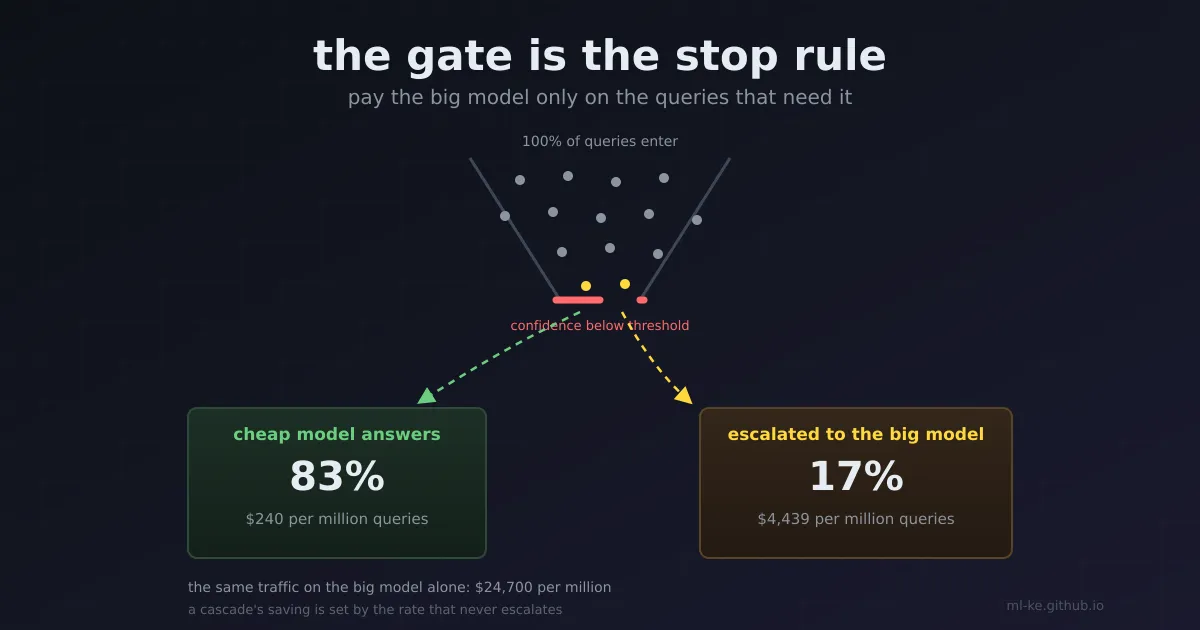
The short version A cascade answers with the cheap model first and only escalates the queries that look unreliable. That idea has real published results behind it: FrugalGPT matched the best single model on one dataset while cutting cost 98 percent, and RouteLLM’s routers reached 95 percent of GPT-4 quality at roughly a quarter of the calls. The arithmetic that decides whether you get those numbers is unglamorous. Cost is almost linear in how much traffic you escalate, so a hundredfold price gap turns every escaped percentage point into real money, and the only thing that keeps the rate low is a score that can tell which queries the big model would fix. Run the small experiment below and one result stands out: at a fixed 20 percent escalation budget, a confidence score recovered 0.426 of the accuracy gap and a perfect score recovered 1.183.
Two models sit behind an API. One costs a hundredth of the other and is right about three quarters of the time. Most products answer that tension by picking one and living with it, which is a decision to overpay on easy traffic or to eat avoidable errors on hard traffic. A cascade refuses the choice: it asks the cheap model first, inspects how confident the answer looks, and pays for the expensive model only on the queries where the cheap one is likely to be wrong.
That description is easy to write and hard to size. The saving is not a property of the architecture, it is a property of your traffic and your stop rule. This post does the arithmetic, runs a planted simulation small enough to finish in a second, then names the two failure modes that delete the savings.
What the published cascades measured
FrugalGPT described the mechanism precisely. A generation scoring function $g(q, a)$ maps a query and a candidate answer to a reliability score in $[0,1]$. The router walks a list of APIs in order, returns the answer when its score clears a threshold $\tau_i$, and queries the next service otherwise. Choosing the list and the threshold vector is a constrained optimisation: maximise expected quality subject to an average cost budget. The paper notes that formulation is mixed-integer and expensive, so it prunes candidate lists whose members rarely disagree and interpolates the objective from a few samples.
The results are worth quoting with their baselines attached, because the headline number travels further than its conditions. On the HEADLINES dataset, GPT-4 scored 0.857 accuracy at a cost of 33.1 units. The learned cascade scored 0.872 at 6.5, which the paper reports as an 80 percent cost cut with a 1.5 point accuracy gain. Table 3 of the same paper asks a different question, namely what it costs to match the best individual model exactly, and answers 33.1 down to 0.6 on HEADLINES (98.3 percent), 9.7 to 2.6 on OVERRULING (73.3 percent), and 72.5 to 29.6 on COQA (59.2 percent). The paper summarises the range as 50 to 98 percent savings. The spread across three datasets is itself the finding: the cascade’s benefit depends on how much of that dataset the cheap model can already handle.
RouteLLM approaches the same problem from the router side. Its routers are trained on preference data, and a single cost threshold $\alpha$ moves the decision: send the query to the weak model when the predicted probability that the strong model wins is below $\alpha$. Because a router that always calls the strong model has perfect quality and zero savings, the paper measures the trade-off in two ways. Performance gap recovered (PGR) is the share of the weak-to-strong accuracy gap a router closes at a given cost. The call-performance threshold, CPT(x), is the fraction of strong-model calls needed to reach x percent of that gap.
At CPT(50) on MT-Bench their best router costs 3.66 times less than GPT-4 while holding 95 percent of its quality, and at CPT(80) the ratio is 2.49. On MMLU the same points are 1.41 and 1.14, with 92 percent of GPT-4 quality at the 50 percent point. On GSM8K, 1.49 and 1.27 at 87 percent. Those figures also carry their working assumption, stated in the appendix: an estimated $24.7 per million tokens for GPT-4 against $0.24 for Mixtral 8x7B. That is the price gap the whole exercise monetises, and it is roughly a hundredfold.
Why a cheap model is worth consulting at all If the cheap model were strictly worse, a cascade could only trade cost for accuracy. FrugalGPT’s complementarity measurement is the reason it can sometimes do both: the maximum performance improvement of one model over another counts the cases where the second is wrong and the first is right. On HEADLINES the inexpensive models could add up to 6 percent over GPT-4 that way, and on COQA 13 percent of items had GPT-4 wrong and GPT-3 right. Routing away from the best single model is not automatically a quality loss.
The bill is close to linear in the escalation rate
Before touching a scorer, write down what a percentage point of escalation costs. If the expensive model costs $G$ times the cheap one, the blended cost per query is $1 + G \cdot r$, where $r$ is the share of traffic that escalates. Nothing about the routing logic changes that shape, which is why a large price gap makes the escalation rate the only number that matters.
1
2
3
4
5
6
7
8
9
10
11
12
SMALL, STRONG = 1.0, 100.0   # same price gap as RouteLLM's per-token estimates

print("escalation rate -> cost index (strong alone = 100) and saving vs strong-alone")
for r in (0.01, 0.05, 0.10, 0.20, 0.35, 0.50, 1.00):
    cost = SMALL + STRONG * r
    print(f"  {r*100:5.1f}%  cost {cost:6.1f}  saving vs strong {100*(STRONG-cost)/STRONG:5.1f}%")

print("\nbreak-even: escalate only when the accuracy gain on that query pays for the gap")
print("required gain in P(correct) = (STRONG - SMALL) / value_of_one_correct_answer")
for value, band in ((10, "never"), (50, "never"), (100, "only a query the cheap model is almost sure to miss"),
                    (500, "hard tail only"), (5000, "most low-confidence queries")):
    print(f"  error costs {value:5d} cheap queries -> need +{(STRONG - SMALL) / value:6.3f} accuracy: {band}")
1
2
3
4
5
6
7
8
9
10
11
12
13
14
15
16
escalation rate -> cost index (strong alone = 100) and saving vs strong-alone
    1.0%  cost    2.0  saving vs strong  98.0%
    5.0%  cost    6.0  saving vs strong  94.0%
   10.0%  cost   11.0  saving vs strong  89.0%
   20.0%  cost   21.0  saving vs strong  79.0%
   35.0%  cost   36.0  saving vs strong  64.0%
   50.0%  cost   51.0  saving vs strong  49.0%
  100.0%  cost  101.0  saving vs strong  -1.0%

break-even: escalate only when the accuracy gain on that query pays for the gap
required gain in P(correct) = (STRONG - SMALL) / value_of_one_correct_answer
  error costs    10 cheap queries -> need + 9.900 accuracy: never
  error costs    50 cheap queries -> need + 1.980 accuracy: never
  error costs   100 cheap queries -> need + 0.990 accuracy: only a query the cheap model is almost sure to miss
  error costs   500 cheap queries -> need + 0.198 accuracy: hard tail only
  error costs  5000 cheap queries -> need + 0.020 accuracy: most low-confidence queries
Read the first table as a budget. Escalating a tenth of traffic already spends 11 percent of the strong model’s bill, and escalating a fifth spends 21. The savings in FrugalGPT’s 98 percent row correspond to a program that escalated a very small share of queries, not to a clever trick inside the cheap model.
The second table is the part most cascade write-ups skip. Escalation is worth it per query only when the expected accuracy gain multiplied by the value of a correct answer exceeds the price gap. At the hundredfold gap, the bar is a full point of accuracy if one error costs as much as a hundred cheap queries. That is a high bar. It means a cascade is a sensible default for consumer chat, internal search, summarisation, and other places where a wrong answer is annoying, and a poor fit for a decision where a wrong answer is expensive, because there the right move is to send the hard queries to the strong model on purpose rather than hope a threshold finds them.
What the stop rule has to accomplish
The score is the only component that decides which queries pay. To see how much it can be worth, plant traffic with known difficulty and compare three ways of spending the same budget.
1
2
3
4
5
6
7
8
9
10
11
12
13
14
15
16
17
18
19
20
21
22
23
24
25
26
27
28
29
30
31
32
33
34
35
36
37
38
39
40
41
42
43
44
45
46
47
48
import random

SMALL, STRONG = 1.0, 100.0
N, SEED, BUDGET = 20000, 7, 0.20


def build(n, seed):
    """Planted traffic: most queries easy, a hard tail. d = difficulty in [0,1]."""
    rng = random.Random(seed)
    rows = []
    for _ in range(n):
        d = rng.random() ** 2
        p_cheap = 1.0 - d ** 1.6
        p_strong = 1.0 - 0.85 * d ** 4.0
        rows.append((p_cheap, p_strong, rng.random() < p_cheap, rng.random() < p_strong))
    return rows


rows = build(N, SEED)
acc_cheap = sum(r[2] for r in rows) / N
acc_strong = sum(r[3] for r in rows) / N


def confidence(rows, noise):
    """The cheap model's own confidence, plus noise. Higher = more sure it is right."""
    rng = random.Random(SEED + 11)
    return [min(1.0, max(0.0, r[0] + rng.gauss(0, noise))) for r in rows]


def accuracy(rows, escalated):
    return sum(rows[i][3] if i in escalated else rows[i][2] for i in range(len(rows))) / len(rows)


k = int(round(BUDGET * N))
conf = confidence(rows, 0.15)
by_conf = set(sorted(range(N), key=lambda i: conf[i])[:k])
rng = random.Random(SEED + 21)
by_random = set(rng.sample(range(N), k))
by_oracle = set(sorted(range(N), key=lambda i: rows[i][3] - rows[i][2], reverse=True)[:k])

print(f"cheap alone   acc {acc_cheap:.3f}  cost {SMALL:5.1f}")
print(f"strong alone  acc {acc_strong:.3f}  cost {STRONG:5.1f}")
print(f"escalating {BUDGET:.0%}: cost {SMALL + STRONG*BUDGET:.1f}, "
      f"{(SMALL + STRONG*BUDGET)/STRONG:.0%} of strong-alone")
for label, chosen in (("random 20%", by_random), ("by confidence", by_conf), ("oracle 20%", by_oracle)):
    a = accuracy(rows, chosen)
    pgr = (a - acc_cheap) / (acc_strong - acc_cheap)
    print(f"  {label:14s} acc {a:.3f}  performance gap recovered {pgr:5.3f}")
1
2
3
4
5
6
cheap alone   acc 0.763  cost   1.0
strong alone  acc 0.906  cost 100.0
escalating 20%: cost 21.0, 21% of strong-alone
  random 20%     acc 0.792  performance gap recovered 0.200
  by confidence  acc 0.824  performance gap recovered 0.426
  oracle 20%     acc 0.932  performance gap recovered 1.183
Random escalation is the null hypothesis and it is not worthless: at 21 percent of the strong model’s cost, random escalation buys 0.792 accuracy against 0.763 for the cheap model alone. That is the floor any router must clear, and it is the reason a cascade with a broken score still looks like it works. The gain comes from the cheap model’s own error rate, not from routing.
Confidence-based escalation doubles that recovery, to 0.426. The arithmetic says the accuracy gap between the two models is 0.143, and a confidence ranking at a fifth of the budget captures about six points of it. It also says most of the remaining gap is still on the table.
The oracle row is the ceiling, and it is above 1.0 on purpose. An oracle that picks the twenty percent of queries with the largest true gain ends at 0.932, higher than the strong model alone, because it also keeps the cheap model’s correct answers on queries the strong model misses. That is FrugalGPT’s complementarity effect appearing in a simulation. For your product the practical consequence is that a well-routed cascade can beat the expensive model rather than merely approximate it, which is exactly the claim in the RouteLLM transfer results and in FrugalGPT’s 4 percent accuracy gain at equal cost.
The gap between 0.426 and 1.183 is where the engineering is. A cascade is a ranking problem, and the ranking you need is not “how unsure is the cheap model” but “how much would the strong model gain here”. Those differ whenever the hard tail defeats both models, which is most of the time in domains where the strong model is also mediocre.
A worse score costs traffic, not accuracy
If you keep the accuracy target fixed and let the escalation rate float, score quality stops being an abstract virtue and becomes a line on the bill. Same planted traffic, four noise levels added to the cheap model’s confidence.
1
2
3
4
5
6
7
8
9
10
11
12
13
14
15
16
17
18
19
20
21
22
23
24
25
26
27
28
29
30
31
32
33
34
35
36
37
38
39
40
41
42
43
44
45
46
47
48
49
50
51
52
53
import random

N, SEED = 20000, 7


def build(n, seed):
    rng = random.Random(seed)
    rows = []
    for _ in range(n):
        d = rng.random() ** 2
        p_c = 1.0 - d ** 1.6
        p_s = 1.0 - 0.85 * d ** 4.0
        rows.append((p_c, p_s, rng.random() < p_c, rng.random() < p_s))
    return rows


rows = build(N, SEED)
acc_c = sum(r[2] for r in rows) / N
acc_s = sum(r[3] for r in rows) / N
target = 0.90 * acc_s


def ranking(rows, noise, seed, overconfidence=1.0):
    rng = random.Random(seed)
    sc = [min(1.0, max(0.0, overconfidence * r[0] + rng.gauss(0, noise))) for r in rows]
    return sorted(range(len(rows)), key=lambda i: sc[i]), sc


def accuracy(order, sc, frac):
    k = int(round(frac * len(order)))
    keep = set(order[:k])
    return sum(rows[i][3] if i in keep else rows[i][2] for i in range(len(rows))) / len(rows)


print(f"cheap {acc_c:.3f}  strong {acc_s:.3f}  target 90% of strong {target:.3f}")
for noise in (0.02, 0.15, 0.30, 0.60):
    order, sc = ranking(rows, noise, SEED + 11)
    lo, hi = 0.0, 1.0
    for _ in range(40):
        mid = (lo + hi) / 2
        if accuracy(order, sc, mid) >= target:
            hi = mid
        else:
            lo = mid
    print(f"scorer noise {noise:.2f}: {hi*100:5.1f}% of traffic escalated to hold the target, "
          f"cost index {1 + 100*hi:6.1f}")

print("\na fixed threshold of 0.50 does not survive a re-calibration of the same scorer:")
for mult, label in ((1.0, "calibrated"), (1.3, "1.3x overconfident")):
    order, sc = ranking(rows, 0.15, SEED + 11, mult)
    k = sum(1 for v in sc if v < 0.50)
    a = accuracy(order, sc, k / len(rows))
    print(f"  {label:18s} escalates {k/len(rows)*100:5.1f}%   cost index {1 + 100*k/len(rows):6.1f}   acc {a:.3f}")
1
2
3
4
5
6
7
8
9
cheap 0.763  strong 0.906  target 90% of strong 0.815
scorer noise 0.02:  16.7% of traffic escalated to hold the target, cost index   17.7
scorer noise 0.15:  17.2% of traffic escalated to hold the target, cost index   18.2
scorer noise 0.30:  20.0% of traffic escalated to hold the target, cost index   21.0
scorer noise 0.60:  25.1% of traffic escalated to hold the target, cost index   26.1

a fixed threshold of 0.50 does not survive a re-calibration of the same scorer:
  calibrated         escalates  20.4%   cost index   21.4   acc 0.825
  1.3x overconfident escalates  14.4%   cost index   15.4   acc 0.806
The noise sweep is the reassuring part. Going from a near-perfect scorer to one whose noise is comparable to the signal moves the escalation rate from 16.7 percent to 25.1 percent, so the cost index moves from 17.7 to 26.1 and the saving versus strong-alone moves from 82 percent to 74 percent. A mediocre scorer leaves most of the win intact, because on traffic where most queries are easy the ranking is dominated by the easy mass. This is why cascades work in practice even when the scorer is crude.
The fixed-threshold result is the uncomfortable part. Multiplying the same confidence by 1.3, which is what a routine prompt tweak or a model upgrade can do, drops escalation to 14.4 percent and accuracy to 0.806, below the 0.815 target the operator believed they had set. Nothing about the ranking changed; the operating point drifted, and a threshold that used to mean “escalate the doubtful fifth” now means something else. A cascade should be configured in escalation rate, measured on a fixed evaluation set, not in score units. If your code says if confidence < 0.7, you have configured a constant that will be wrong after the next model swap for reasons nobody instruments.
The two traps that erase the saving
The first trap is a router that needs both answers to decide. If your routing rule compares the cheap and strong outputs, or grades the cheap output with the strong model, you have already paid for the strong model on every query.
1
2
3
4
5
6
7
8
9
10
11
12
13
14
15
16
17
18
19
20
21
STRONG_PER_MTOK = 24.7   # RouteLLM appendix D estimate for GPT-4-class
CHEAP_PER_MTOK = 0.24    # same appendix, Mixtral 8x7B-class
ROUTER_PER_MREQ = 3.19   # RouteLLM table 7, BERT router
TOKENS_PER_QUERY = 1000  # 700 in + 300 out: this post's assumption, not theirs
ESCALATION = 0.17        # measured in the block above

queries = 1_000_000
mtok = queries * TOKENS_PER_QUERY / 1_000_000
strong = mtok * STRONG_PER_MTOK
cheap = mtok * CHEAP_PER_MTOK
cascade = cheap + ESCALATION * strong
agreement = strong + cheap
router = queries / 1_000_000 * ROUTER_PER_MREQ

print(f"per {queries:,} queries at {TOKENS_PER_QUERY} tokens each = {mtok:,.0f} M tokens")
print(f"  strong alone          ${strong:9,.0f}")
print(f"  cheap alone           ${cheap:9,.0f}")
print(f"  cascade at {ESCALATION:.0%}      ${cascade:9,.0f}   ({100*(strong-cascade)/strong:.1f}% below strong-alone)")
print(f"  run both, decide after ${agreement:9,.0f}   ({100*(agreement-strong)/strong:+.1f}% vs strong-alone)")
print(f"  a BERT-class router costs ${router:,.2f} per million requests = "
      f"{100*router/strong:.4f}% of the strong bill")
1
2
3
4
5
6
per 1,000,000 queries at 1000 tokens each = 1,000 M tokens
  strong alone          $   24,700
  cheap alone           $      240
  cascade at 17%      $    4,439   (82.0% below strong-alone)
  run both, decide after $   24,940   (+1.0% vs strong-alone)
  a BERT-class router costs $3.19 per million requests = 0.0129% of the strong bill
Running both models and deciding afterwards costs $24,940 per million queries, one percent more than using the strong model for everything. The cascade costs $4,439. The difference between those two rows is the whole discipline of routing: the decision has to be made from the query alone, before the expensive generation is paid for. RouteLLM’s router overhead measurements make the same point from the other side. Their BERT classifier costs $3.19 per million requests at 69 requests per second, a rounding error against the generation bill, while a causal-LLM router costs $5.23 and does 42 requests per second.
The second trap is scaling the score instead of an operating point. A cascade shipped with a fixed threshold and no escalation-rate monitor can pass every test and still lose money, because the rate is what the bill reads. Log the escalation decision, the score that produced it, and the eventual outcome, then watch the rate weekly. If the rate moves without a deliberate change, the scorer moved.
Sizing a cascade before you ship it
Each step below produces a number you can put in a design document, and any of them can end the project early.
- Measure the per-query accuracy gap on your own traffic, not on a public benchmark. Two hundred to a few thousand labelled items from the real distribution is enough to start, and the gap on your tail will be smaller than the gap on someone else’s benchmark.
- Fix the value of a correct answer in cheap-query units. If one error costs the equivalent of 100 cheap queries, the break-even table above says escalation needs a full point of accuracy to pay for itself per query. That number decides whether a cascade is appropriate at all.
- Compute the cost line before building the router. At a hundredfold price gap, cost is $1 + 100r$. Decide the maximum escalation rate you are willing to pay for, and treat it as a budget rather than a result.
- Score the queries, not the confidence. Where you have labels, fit a small model on features available before the expensive call, such as the cheap model’s mean token log-probability, answer length, retrieval score, and self-consistency across a few cheap samples. Then measure PGR at your budget and compare it against the random-escalation floor on the same traffic.
- Set the threshold in rate units and monitor it. Pick the cut that escalates your budgeted percentage on the evaluation set, store the rate as a metric, and alert when it drifts by more than a few points. The 1.3x recalibration above is what silent drift looks like.
- Feed the escalated cases back. The escalated set is a labelled sample of your hardest traffic, which is exactly the data worth fine-tuning the cheap model on. FrugalGPT’s second strategy, model approximation, is that loop, and it is how the escalation rate comes down over time rather than rising.
On a hundredfold gap, a cascade’s saving is dominated by how much traffic never escalates, so resist tuning accuracy upward by raising the rate. The comparison is never cascade versus cheap model. It is cascade versus the strong model at the accuracy you need, on traffic you have.
Key takeaways
| Question | Measured answer | What it means |
|---|---|---|
| What does escalation cost? | $1 + 100r$ at the published price gap: 10 percent traffic costs an 11th of the strong bill, 20 percent costs a 21st | Cost is set by the rate, not the architecture |
| When is escalating one query worth it? | Needs a 0.198 accuracy gain if an error costs 500 cheap queries, 0.990 if it costs 100 | Cascades suit low-stakes answers, not expensive decisions |
| How much does the score buy at 20 percent? | Random 0.200 of the gap, confidence 0.426, oracle 1.183 | The stop rule, not the price gap, is the engineering |
| What does a noisy score cost? | Escalation rises 16.7 percent to 25.1 percent to hold 90 percent of strong accuracy | A worse scorer costs money, not accuracy |
| What does a fixed threshold cost? | A 1.3x recalibration moves escalation from 20.4 to 14.4 percent and accuracy from 0.825 to 0.806 | Configure a rate, monitor the rate |
| What if the router sees both answers? | $24,940 versus $4,439 per million queries | Decide before you pay for the strong model |
References
- Chen, Zaharia, Zou, FrugalGPT: How to Use Large Language Models While Reducing Cost and Improving Performance, arXiv:2305.05176, May 2023. The generation scoring function and threshold router in section 3, the constrained formulation, the HEADLINES case study at 0.857 versus 0.872 accuracy and 33.1 versus 6.5 cost, Table 3 for the 98.3, 73.3 and 59.2 percent matching costs, and the complementarity figures of 6 percent on HEADLINES and 13 percent on COQA.
- Ong et al., RouteLLM: Learning to Route LLMs with Preference Data, arXiv:2406.18665v4, ICLR 2025. The cost threshold in section 3.2, the PGR, APGR and CPT definitions, Table 6 for 3.66 and 2.49 on MT-Bench, 1.41 and 1.14 on MMLU, 1.49 and 1.27 on GSM8K, the $24.7 versus $0.24 per million token estimates in appendix D, and Table 7 for router overhead.
Related posts
- Is Your +3-Point Eval Gain Real? Gating a Comparison with Paired Statistics — the test to run before treating an escalation-rate change as an improvement.
- Agreement Before Accuracy: Auditing the Labels You Are About to Train On — the label quality behind the accuracy gap a cascade is trying to recover.
- Probability Calibration for Risk Scores — why a confidence number can rank well and still be the wrong threshold.
- A Semantic Cache Only Saves Money Above a Threshold You Measured — the other way to cut the strong model’s bill, and the same threshold discipline.
- Rank Is a Budget: What LoRA at r=8 Costs and Buys on an 8B Model — the same move on the training side, where the budget is parameter count.